O.Tarasov 1, D.Bazin 2, O.Sorlin 3, M.Lewitowicz 4
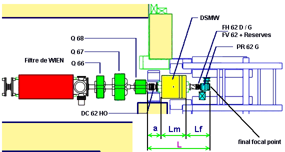
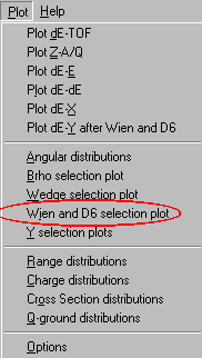
2. Dipole D6 after the Wien Filter
1. Introduction (brief description of previous series)
The program 1) called after the spectrometer LISE 2) has been developed in GANIL (Caen, France) to calculate the transmission and yields of fragments produced and collected in an achromatic spectrometer. This code allows to simulate an experiment, beginning from the parameters of the reaction mechanism and finishing with the registration of products selected by a spectrometer. The program allows to quickly optimize the parameters of the spectrometer before or during the experiment. It also makes it possible to estimate and work in conditions of maximum output of studied reaction products and their unambiguous identification.
Wedge and Wien filter selections are also included in the program. In-built Energy loss, Time-of-Flight, Position, Angular, Charge, Cross-Section distribution plots and dE-E, dE-TOF and Z-A/Q two-dimensional plots allow to visualize the results of the program calculations.
An application of transport integral 3) lies in the basis of fast calculations of the program for the estimation of temporary evolution of distributions of phase space.
Recently in the frame of the collaboration Dubna-GANIL the program has undergone a number of serious changes and has been adapted to the environment of "Windows":
It is possible to receive this program and the last version for MS-DOS using FTP to the address (user: anonymous):
2. Dipole D6 after the Wien Filter
![]() The dipole D6
is placed on the turning platform in a vertical plane behind the Wien Filter.
The dipole radius is determined as R @Lm
/ q , where q is
the angle of platform turning. Angle may be varied from 0 up to 23 degrees.
This dipole (denoted as DSMW on the Fig.1) serves for the fourth selection
on the mass and the charge of nucleus (A/Q). Selection by this dipole as
the Filter Wien is performed in a vertical plane.
The dipole D6
is placed on the turning platform in a vertical plane behind the Wien Filter.
The dipole radius is determined as R @Lm
/ q , where q is
the angle of platform turning. Angle may be varied from 0 up to 23 degrees.
This dipole (denoted as DSMW on the Fig.1) serves for the fourth selection
on the mass and the charge of nucleus (A/Q). Selection by this dipole as
the Filter Wien is performed in a vertical plane.
2.1. Angle of platform
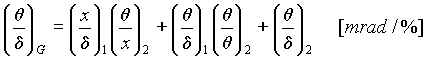
The angle of platform turning is calculated from the optical conditions and as much as possible to compensate the filter velocity dispersion to get only A/Q dispersion at the focal point after turning dipole. The Wien filter optical structure supposes that six focalization conditions must be fulfilled to have the best matching at the detection location. With addition of the turning dipole D6 these conditions must be saved. To find the angle of turning it is necessary to solve the following equation (given by R.Anne) arising from optical conditions:
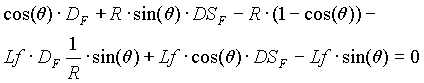 , [1]
, [1]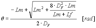 . [2]
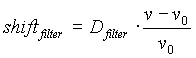
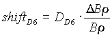
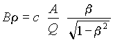
. [2]The image shift of nuclei in the final focus plane can be roughly determined in the following way :
 , [4]
, [4]
 , [5]
, [5]
Using equation
 , [6]
, [6]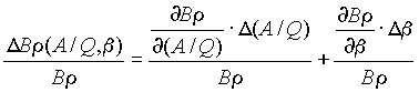 [7]
[7]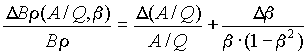 . [8]
. [8]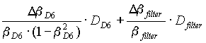 [9]
[9]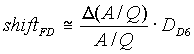 [10]
[10]Some possible combinations are considered in the program :
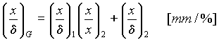
The image size (distribution) defined in the program LISE is a result of convolution of two distributions PY and PY :
 , [12]
Repeating all steps like in the previous section it is possible to conclude
that the use of the "fd-system" supposes that Pd/Y
vanishes because as it was metioned before the sum (equation 9) is
close to 0 and the value D (A/Q) for an isotope
relatively itself is equal 0. It means that the final Y-image will be narrower,
thus providing a better resolution than in the simple case of the velocity
filter only. Hence the second distribution is taken as the d
-function in order to get ![]() as a result of convolution.
as a result of convolution.
After this consideration it is possible to compare the fd-system with an ordinary velocity filter (see Table 1) : application of the fd-system provides better results for smaller object size and wider momentum distribution.
Table 1.
|
|
degrader in LISE |
degrader in ALPHA |
|
|
|
|
|
|
|
|
|
|
|
|
|
|
|
|
|
|
|
|
|
|
|
|
|
|
|
|
|
|
|
|
|
|
|
|
|
|
|
|
|
|
|
|
|
|
|
|
|
|
|
|
|
|
|
|
|
|
|
|
|
|
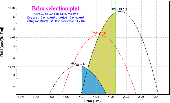
2.4. Separation with the Dipole D6
The LISE standard configuration was chosen in order to compare different modes of selection. These experimental settings (beam, target, wedge, slits) are given below.
Fig.2.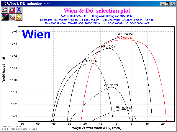
Fig.3. 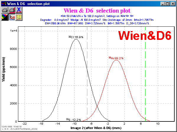
| Mode |
|
|
|
|
|
|
| 1 | First dipole |
|
|
|
|
|
| 2 | 1 + Wedge |
|
|
|
|
|
| 3 | 2 + Wien Filter |
|
|
|
|
|
| 4 | 3 + D6-dipole |
|
|
|
|
|
The advantage of using all 4 selections follows apparently from Table 2. In this case the purification is 30 times better than after the first selection, but the 36Ar rate is lower only in 1.5 times. Figures 2 and 3 show vertical space distributions in the focal final plane for selections by the velocity filter and the fd-system. The contribution of momentum distribution into the vertical image due to existence of non-zero velocity dispersion in the mode only with the velocity filter (Fig.2) makes the image wider as compared to the fd-system that was already discussed in §2.3. image size.
2.5. The program LISE for the new spectrometer VAMOS
VAMOS 10) is a collaboration to build a large acceptance spectrometer for identifying products of reactions induced by the Systeme de Production d'Ions Radioactifs et d'Acceleration en Ligne (SPIRAL) facility at the Grand Accelerateur National d'Ions Lourds (GANIL).
The QQFD-spectrometer VAMOS has the following main properties and characteristics:
Version 3.4
[general]
File = C:\LISE\config\VAMOS.lcf
Date = 12-05-1999
Time = 13:41:31
Title = VAMOS
[object]
X Slits before target = 10 (±)mm ; hor.slit
width before target to collimate a beam
Y Slits before target = 10 (±)mm ; ver.slit
width before target to collimate a beam
X Slits intermediate = 100 (±)mm ; hor.slit
width at the dispersive focal plane
Y Slits intermediate = 10 (±)mm ; ver.slit
width at the dispersive focal plane
X Slits first focus = 10 (±)mm ; hor.slit
width at the first focal point /after wedge/
Y Slits first focus = 10 (±)mm ; ver.slit
width at the first focal point /after wedge/
Slits second focus = 10 (±)mm ; ver.slit width
at the second focal point /after Wien/
[acceptances]
Maximal momentum accept = 5 (±)% ; upper limit
for the setting of the slits
Theta target acceptance = 160 (±)mrad ; angular
target horiz.acceptance
Theta wedge acceptance = 200 (±)mrad ; angular
wedge horiz.acceptance
Phi target acceptance = 160 (±)mrad ; angular
target vert.acceptance
Phi wedge acceptance = 200 (±)mrad ; angular
wedge vert.acceptance
[optics]
BX = 1.5 (±)mm ; one-half the horisontal beam
extent (x)
BT = 3.3 (±)mrad ; one-half the horisontal
beam divergence(x')
BY = 1.5 (±)mm ; one-half the vertical beam
extent (y)
BF = 3.3 (±)mrad ; one-half the vertical beam
divergence (y')
BD = 0.1 (±)% ; one-half of the momentum spread
(dp/p)
Ra1 = 2.6 m ; Curvature radius of first dipole
Ra2 = 2.003 m ; Curvature radius of second dipole
L target-wedge = 0 m ; Object - DispFocPlane
L wedge-detector#1 = 0 m ; DispFocPlane-AchrFinalPlane
M1X = 1 ; X Magnification target -> wedge
D1X = 10 mm/% ; X dispersion target -> wedge
M1T = 1 ; theta magnific. target -> wedge
D1T = 0 mrad/% ; theta dispers. target -> wedge
ThX = 0.1 mrad/mm ; theta/x coef. target -> wedge
M1Y = 1 ; Y Magnification target -> wedge
PhY = 0.1 mrad/mm ; fi/y coef. target -> wedge
M1P = 1 ; fi magnificat. target -> wedge
M2X = 1 ; X Magnification wedge -> focal
D2X = -10 mm/% ; X dispersion wedge -> focal
M2T = 1 ; theta magnific. wedge -> focal
D2T = -1 mrad/% ; theta dispers. wedge -> focal
T2X = 0.1 mrad/mm ; theta/x coef. wedge -> focal
M2Y = 1 ; Y Magnification wedge -> focal
P2Y = 0.1 mrad/mm ; fi/y coef. wedge -> focal
M2P = 1 ; fi magnificat. wedge -> focal
Angle = 0 mrad ; beam respect to the spectrometer
axis
[wien_filter]
Wien filter = Enabled ; Disabled & Enabled
E_F = 2000 kV/m ; electric field
B_F = 478.861416 G ; magnetic field
DiC = 1.3856e-3 mm/% ; dispersion coefficient
LenE = 1 m ; effective electric length
LenB = 1 m ; effective magnetic length
Red = 1 ; Real/Red field
Mag = 1 ; Magnification
3.1. Physical calculator
![]() Very often it is necessary
for User to perform a fast transformation of one physical value to another
while working with the program. The dialog GOODIES allows to get calculated
correlated value only for a given Br -value
obtained for a setting fragment. However, if User needs to know (for example)
a range in some material for energy unconnected with given settings? The
new version of the code LISE allows to solve this problem. The new dialog
Physical calculator permits immediately to perform calculations of correlated
values independently from calculations for a setting fragment. Clicking
on any radiobutton User may choose the respective form to type a physical
value in order to get other correlated values. For example, User may input
the Br -value for 36Ar (see Fig.4)
and get all correlated values including the range in the given material
and the energy loss for the chosen thickness, or typing the energy rest
22Al
after the material (Si 100 mg/cm2 in Fig.4), one can recalculate
initial energy of a nucleus before the material and other correlated values
as shown in Fig.5.
Very often it is necessary
for User to perform a fast transformation of one physical value to another
while working with the program. The dialog GOODIES allows to get calculated
correlated value only for a given Br -value
obtained for a setting fragment. However, if User needs to know (for example)
a range in some material for energy unconnected with given settings? The
new version of the code LISE allows to solve this problem. The new dialog
Physical calculator permits immediately to perform calculations of correlated
values independently from calculations for a setting fragment. Clicking
on any radiobutton User may choose the respective form to type a physical
value in order to get other correlated values. For example, User may input
the Br -value for 36Ar (see Fig.4)
and get all correlated values including the range in the given material
and the energy loss for the chosen thickness, or typing the energy rest
22Al
after the material (Si 100 mg/cm2 in Fig.4), one can recalculate
initial energy of a nucleus before the material and other correlated values
as shown in Fig.5.
The eight correlated values of a nucleus (which is inputted in the upper part of the dialog) are included to Physical calculator:
3.2. Configuration file
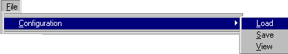
Two types of files were used in the previous version of the program : LISE-file (extension LIZ) and Result-file (extension RES). The data settings could be recovered only from LISE-files. If User wanted to repeat old settings for a new file it was necessary first to find the corresponding LISE-file with same setup configuration and then to save it with a new name. In the new version there is an additional possibility to save and to extract settings to/from the new kind of file is called Configuration-file. User has an access to these files via the menu File -> Configuration. These files contain only some divisions from standard LISE-file :
On the base of optical matrices and physical characteristics of setups given in the Ref.11,10), different setups for the LISE program were put to configuration files. User may find these configuration files in the distributive version lise34.zip :
3.3. Angle for Thickness
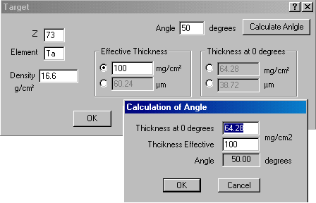
![]() Physicist
may vary a target thickness changing an angle of target that is placed
into the target box of the SISSI device or the LISE spectrometer. Sometimes
it is necessary to calculate and input the value of the angle in the experiment.
In the new version of the code User can change an angle of a target (wedge,
degrader, materials). There is a possibility to calculate each of three
values from the two other known ones : Effective thickness, Thickness at
0 degrees or Angle of turning (see Fig.7). For example, if User knows the
effective target thickness and the thickness at 0 degrees he can simply
click on the button Calculate Angle to get the angle value as shown
in Fig.7. User may input the material thickness using two dimensions :
mg/cm2 or microns.
Physicist
may vary a target thickness changing an angle of target that is placed
into the target box of the SISSI device or the LISE spectrometer. Sometimes
it is necessary to calculate and input the value of the angle in the experiment.
In the new version of the code User can change an angle of a target (wedge,
degrader, materials). There is a possibility to calculate each of three
values from the two other known ones : Effective thickness, Thickness at
0 degrees or Angle of turning (see Fig.7). For example, if User knows the
effective target thickness and the thickness at 0 degrees he can simply
click on the button Calculate Angle to get the angle value as shown
in Fig.7. User may input the material thickness using two dimensions :
mg/cm2 or microns.
3.4. List of recently used files
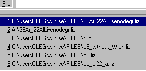
To open a document User has used recently, it is necessary to click
its name at the bottom of the File menu where the list of recently used
documents is placed.
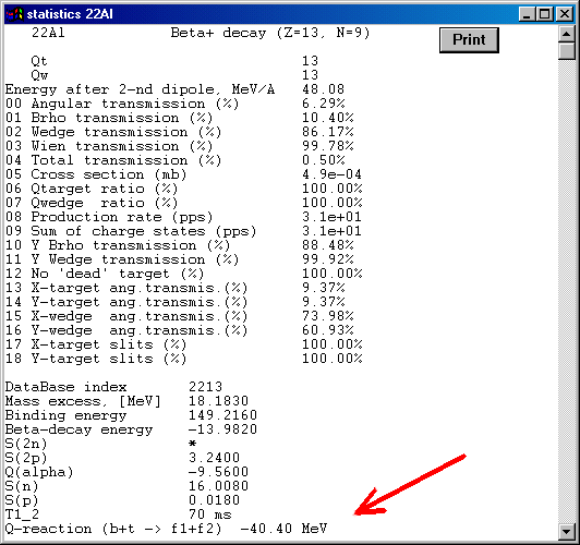
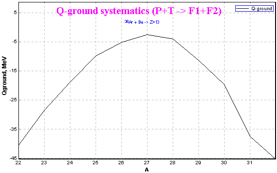
3.5. Calculation of Q-ground value for binary reaction
In the new version User may see a Q-value of reaction at the bottom of the window Statistics (this window is appeared when User clicks on an isotope of interest in the table of nuclides by the right button of the mouse). Q-value is calculated from the supposition that the reaction has two nuclei as a result. The first nucleus is the nucleus chosen by User, the second one is calculated as residual from Projectile + Target - Fragment of Interest . Therefore Q-value is estimated as :
3.6. Chromatic mode (Dispersion ¹ 0)
![]() Since its
first version, the program has been adapted to operate only in the achromatic
mode. The focal plane of the second section being achromatic, there is
no momentum dependence of the final horizontal position (as well as vertical).
In the new version the admission that the full momentum dispersion is not
equal to 0 has been included. User may observe this admission on the Wedge
image (X) plot in the First focal plane. This assumption is fulfilled because
the selection by the velocity filter and the dipole D6 takes place in
the Y-plane. Using this new mode User may visualize the images and obtain
a transmission not only for ideal case of an achromatic spectrometer.
Since its
first version, the program has been adapted to operate only in the achromatic
mode. The focal plane of the second section being achromatic, there is
no momentum dependence of the final horizontal position (as well as vertical).
In the new version the admission that the full momentum dispersion is not
equal to 0 has been included. User may observe this admission on the Wedge
image (X) plot in the First focal plane. This assumption is fulfilled because
the selection by the velocity filter and the dipole D6 takes place in
the Y-plane. Using this new mode User may visualize the images and obtain
a transmission not only for ideal case of an achromatic spectrometer.
The code is calculated full momentum and angular dispersions on the base of inputted in the program the two transport matrices for both parts of the spectrometer as :
 ,
[14]
,
[14]
 . [15]
Fig.09. 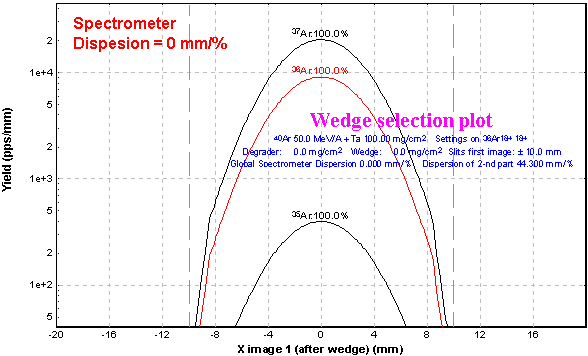
Fig.10.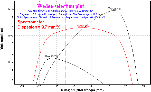
4.1. Results file
The Results file has not been changed since its DOS-version 2.5, and consequently in versions 3.0-3.3.05 it does not reflect all parameters needed for User (D6-dipole parameters, applied methods of the cross-section parameterization and the ionic charge state distributions, target angle). In the new version the Results file has got more readable form, and all values needed for further work of User with this file have been included.
LISE CALCULATIONS Version 3.4
File : C:\user\OLEG\winlise\FILES\36Ar_22AlLisenodegr.liz
Date : 5/19/1999 Time : 9:13:01
Title : 22Al
Projectile : 36Ar 18+ at 94.4
MeV/u - Intensity : 1000 enA
Target : Be Thickness : 537.95
mg/cm2 (2907.84 microns)
Wedge : Be Thickness : 196.47
mg/cm2 (1062 microns)
Material(s) :
#1 : Si Thickness : 69.9 mg/cm2
(300 microns)
#2 : Si Thickness : 69.9 mg/cm2
(300 microns)
#4 : Si Thickness : 116.5 mg/cm2
(500 microns)
#5 : Si Thickness : 116.5 mg/cm2
(500 microns)
#6 : Si Thickness : 1398 mg/cm2
(6000 microns)
Settings calculated on 22Al
13+ 13+
Brho1=1.9530 Tm Brho2=1.7100
Tm (B1=0.7512 T B2=0.8537 T)
Wien filter : E=3500.0 kV/m
B=331.8000 G Disp=3.184 mm/% Magn=1
D6 : B=0.5354 T Angle=13.97
deg Disp=3.185 mm/%
Mechanism: Vopt/Vbeam=1.000
Sigma0=90.0 MeV/c SigmaD=200.0 MeV/c
Methods: Cross Section=0 Charge
states=0
Acceptances :
Maximum momentum acceptance
: +/- 2.50 %
Target : Theta : +/- 17.45 mrad
Phi : +/- 17.45 mrad
Wedge : Theta : +/- 20.26 mrad
Phi : +/- 6.00 mrad
Slits :
X,Y Slits before target (Collimator)
mm +/- : 15 15
X,Y Slits intermediate (Momentum
sel.) mm +/- : 8.6 10
% in Brho +/- : 0.50
X,Y Slits first focus(Wedge
selection) mm +/- : 7 10
Second image slits (Wien selection)
mm +/- : 5
Beam emittance (+/-): 1.5 mm
3.3 mrad 1.5 mm 3.3 mrad 0.1 %
Beam angle on target : 0 mrad
OPTICS ([mm],[mrad]):
Target - DispFocalPlane(Wedge)
DispFocalPlane(Wedge)-First image
-0.783 * * * 17.3 -2.5607 *
* * 44.3
0.267 -1.284 * * 3.51 0.4 -0.389
* * -5.56
* * -4.26 * * * * -0.432 * *
* * -0.858 -0.273 * * * -0.32
-2.4 *
TRANSMISSION AND RATE CALCULATIONS
A Z |Qt |Qw | Ang. | Brho |Wedge
|WienD6|Y&C&DT| Total | Cross | Rate | Qt | Qw
| | |Trans.|Trans.|Trans.|Trans.|Trans.|
Trans.|Section| | |
| | | (%) | (%) | (%) | (%)
| (%) | (%) | (mb) | (pps) | (%) | (%)
-----|---|---|------|------|------|------|------|-------|-------|-------|------|-----
23Si| | | 6.534| 4.692| 85.05|
2.641| 88.41| 0.0061|3.3e-06| 0.0025| |
22Al| | | 6.291| 10.40| 86.17|
99.78| 88.41| 0.4972|0.00049| 31| |
21Mg| | | 6.018| 4.905| 84.89|
0.921| 88.41| 0.0020| 0.029| 7.5| |
================================================================================
ALMOST : 38 pps
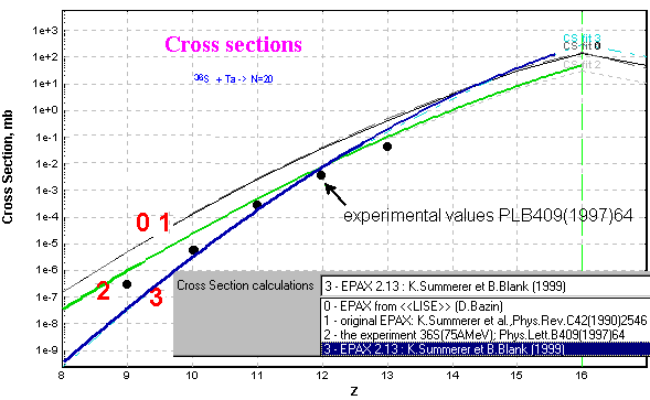
4.2. New parameterization
![]() The code used
three in-built parameterizations of cross-sections on the EPAX 4)
base. The new parameterization EPAX 2.13 has been kindly presented by B.Blank
and K.Summerer for the new LISE-version. This new approximation shows very
good agreement in cross-section estimation for proton rich fragments, while
for the super neutron rich isotopes placed far from a beam 12)
the discrepancy appears (see Fig.12) as in the previous parameterization
but from the other side.
The code used
three in-built parameterizations of cross-sections on the EPAX 4)
base. The new parameterization EPAX 2.13 has been kindly presented by B.Blank
and K.Summerer for the new LISE-version. This new approximation shows very
good agreement in cross-section estimation for proton rich fragments, while
for the super neutron rich isotopes placed far from a beam 12)
the discrepancy appears (see Fig.12) as in the previous parameterization
but from the other side.
User may choose the new parameterization to perform calculations via
the Menu
Options->Production Mechanism.
4.3. Trigonometric function of the in-built calculator
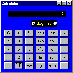
![]() The trigonometric functions (sin, cos, tan, arcsin, arccos) have
been added in the in-built calculator. User has also got an opportunity
to choose units (degrees or radian) for trigonometric calculations (see
Fig.13).
The trigonometric functions (sin, cos, tan, arcsin, arccos) have
been added in the in-built calculator. User has also got an opportunity
to choose units (degrees or radian) for trigonometric calculations (see
Fig.13).
4.4. Three points interpolation for the energy loss and range subroutines

5. Plots
5.1. image after Wedge & D6 (one-dimensional
plot) and dE - Y image (after wedge & D6)
 |
The two-dimensional plot (right menu) dE-Y (Energy Loss versus Y-image) is presented in Fig.15.
|
 |
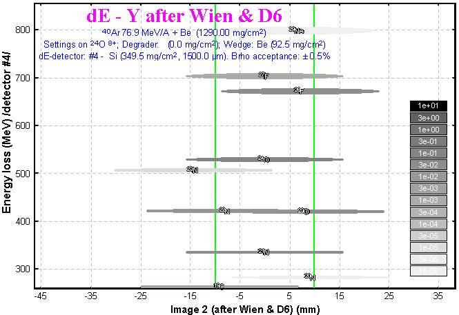
Fig.16.
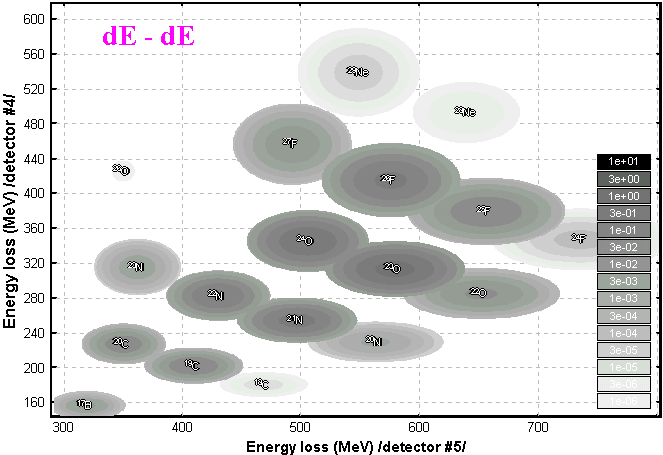
5.2. dE-dE plot
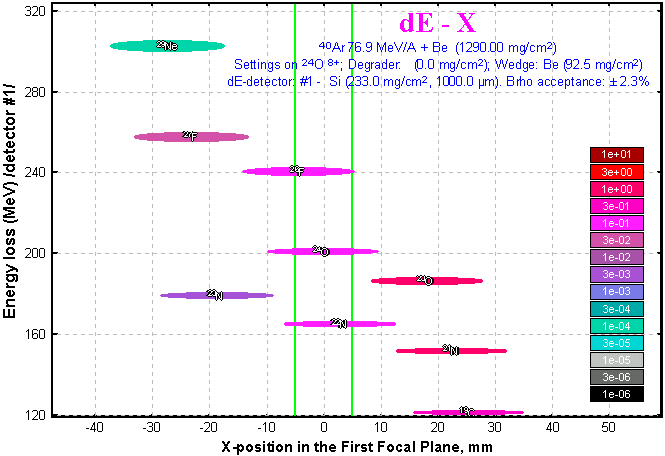
5.3. dE-X plot
5.4. Plot of Q-ground values
5.5. Realistic image of peaks
![]() Two-dimensional
plots in standard mode are drawn only by one color corresponding to their
intensity. The width of peak is equal to its distribution FHWM. Realistic
mode for peak drawing uses some colors depending on a distance between
the peak center and given point inside the peak (width ±
2s ). Example of the plot drawn in the realistic
mode is presented in Fig.17.
Two-dimensional
plots in standard mode are drawn only by one color corresponding to their
intensity. The width of peak is equal to its distribution FHWM. Realistic
mode for peak drawing uses some colors depending on a distance between
the peak center and given point inside the peak (width ±
2s ). Example of the plot drawn in the realistic
mode is presented in Fig.17.
5.6. Gray and Color Palettes for two-dimensional plots
![]() User does
not always have a possibility to print two-dimensional plots on color printers.
Therefore the button has been added to switch the palettes of plot to reproduce
intensity of peak for printing.
User does
not always have a possibility to print two-dimensional plots on color printers.
Therefore the button has been added to switch the palettes of plot to reproduce
intensity of peak for printing.
6.1. The thickness dialog - density
Before it was impossible to input a float value into the density window of the thickness dialog. This has been corrected.
6.2. The dialog Calibrations
After inputting new nucleus in the calibrations dialog the range was not recalculated. This has been corrected.
6.3. Adaptation the code to the PC emulator on Mac
Cross-section calculations were performed incorrectly on Mac under the PC-emulator due to some discrepancy in the C function pow(x,y) between these system platforms (?). The function pow(x,y) has been changed in the code by redefinition #define pow(x,y) exp((y) log(x))
6.4. Negative dispersion
The negative momentum dispersion provoked a crash of the program. This has been corrected and User may use the negative momentum dispersion.
6.5. After reading of a LISE-file the program did not calculate magnetic field
The conjugate values (Br and B) are immediately recalculated when User changes the Br-values or the B(magnetic field)-values using the dipoles dialog or when the program calculates these values. When User read a LISE-file, the Br-values were inputted into the code but without recalculation of the magnetic field. This has been corrected.
6.6 Distributions
Some bugs provoking crash of the program have been corrected.
2) R.Anne et al., NIM A257(1987) p.215-232; Web-site of the LISE
spectrometer:
http://www.ganil.fr/LISE.
3) D.Bazin and B.Sherrill, Phys.Rev. E50(1994) 4017-4021.
4) K.Sümmerer et al., Phys.Rev. C42(1990)2546-2561.
5) O.Tarasov et al., Nucl.Phys. A629(1998)605.
6) A.Leon et al., Atom.Data and Nucl.Data Tables, v.69, 1998.
7) THE 1995 ATOMIC MASS EVALUATION, G.Audi and A.H.Wapstra, Atom.Data and Nucl.Data Tables (1995).
8) The code NUCLEUS - I.Duflo, G.Audi et al, CSNSM, Orsay
9) Transport: a computer program for designing charged particle beam transport system, K.L.Brown, D.C.Carey, Ch.Iselin, F.Rothacker. CERN 80-04.
10) VAMOS: WEB-reference http://www.ganil.fr/vamos/index.html.
11) Guide de lutilisateur de SISSI, M-H.Moscatello et le groupe SISSI, GANIL R96 05 ;. WEB-refernce http://www.ganil.fr/equipements/equip_detect.htmlx.