THE
CODE
LISE:
new versions 4.14, 4.15
East
Lansing
23-MAR-2001
Plot calibration utilities
NSCL & The LISE code
Contents:
1.
Plot calibration utilities version 4.15
1.1.
Calibration of physical parameters
1.2.
Two-dimensional plots in the calibration mode
1.3.
New options of plots
2.1.
Calibration of A1900s dipoles
2.2.
Support of NSCL specters
2.3.
Balls animation for Windows NT
2.4.
Optimization of Monte-Carlo plots
1.Plot
calibration utilities version 4.15
Physics get in experiments the data in relative channels,
then translate them proceeding from given calibration in real physical
values. On the contrary the program does all calculations and creates the
plots in absolute physical values. For comparison of calculations with
experimental data a physicist was obliged with the calculator quickly to
recalculate these plots. In the old versions under DOS the program allowed
to deduce in channels for the plot dE-TOF. In the new version of the program
it has been incorporated a possibility to input calibrations of 7 materials(detectors)
and next 4 parameters: time of flight (TOF), total kinetic energy (TKE),
horizontal distributions in disperse and final focal planes. All calibration
values are kept in LISE-files.
1.1.Calibration
of physical parameters
Calibration
values for materials (detectors) are entered through the dialogue "Material",
then the button "Calibration". The user can enter given as calibration
of physical values through channels, so channels through physical values
with the help of switching of a direction of input (see Fig.1). A name
of dimension of physical value also can be modified (in the given figure
the dimension is "MeV").
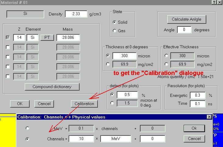
Fig.1.
Input of calibration values of a material (detector).
Input of calibration values for parameters TOF, TKE,
Xdisp, and Xfinal is carried
out through the dialogue Plot options (menu Plots)(see
Fig.2 , the box A).
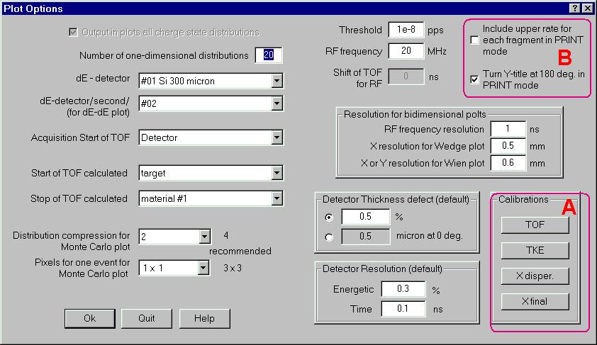
Fig.2.
The dialogue Plot options. The box A is showing the panel for input of
calibration values for parameters TOF, Tke, Xdisp, Xfinal. The box B is
showing new options to printplots.
1.2.Two-dimensional
plots in the calibration mode
At work with
two-dimensional plots a new window exists in the new version, where the
relative channels values are displayed on the basis of entered calibrated
values (see A in Fig.3). This innovation works as well as standard mode,
and with Monte-Carlo method. Also all calibration values are transformed
and in case of change of a direction of a horizontal axis, or change of
axes X and Y.
Fig.3.
The bi-dimensional plot dE-TOF. New calibration possibilities are marked
by arrows. For details see the text.
The user can change
calibration values directly at work with the given plot, pressing on an
icon that is shown by the arrow C in Fig.3. As a result of this action
there is the dialogue Plot's Calibration. Besides that the user can change
calibration, he also can put an option, that the axes were in channels
designed on the basis of calibration that facilitate comparison of the
experimental plots with designed by the program LISE. If the user has chosen
an option of a conclusion given in channels, there is an inscription Channels
in red color, and the digits on an axis also are deduced in red color (see
Fig.3, arrow B)
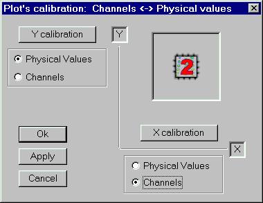
Fig.4.
The dialogue Plots calibration allows to change calibration values
and to choose a method to draw axiss values (physical
values or channels).
1.3.New
options of plots
In the early versions of the LISE program a fragment
rate was always typed also to the right of a fragment name
at output of two-dimensional plots on a printer. It was caused
by that it were earlier used black-and-white printers to print. Now color
printers are used everywhere. The user can switch off this possibility
and print a plot without rates value (see Fig.2, box B).
Unfortunately, the vertical inscriptions for various
systems are deduced on the printer not as they are visible on the screen.
The inscriptions are developed on 180 degrees sometimes in PRINT mode.
To explain it was more hardly, than to make simply option of turn of the
name of a vertical axis in PRINT mode (see Fig.2, box B). So for GANIL
and JINR
this option should be switched off, and for NSCL is on the contrary included.
However user always can himself check up and choose an option inherent
for his system.
2.NSCL
& The LISE code - version
4.14
The user may
get the scheme of new A1900 spectrometer using the menu Help -> A1900
spectrometer.
2.1.Calibration
of A1900s dipoles
As well as for setups LISE and M5678 (JINR) the calibration
values of magnetic dipoles were entered for the A1900 spectrometer. Through
the menu Utilities -> A1900 calibration <PLAN> the User may
get the scheme of the A1900 spectrometer, where he can with the help of
buttons choose a necessary dipole. The values can be entered as in tesla-meters,
tesla, and ampers at the request of the user.
Fig.5.
The A1900 spectrometer scheme with dipole calibration buttons.
2.2.Support
of NSCL specters
In
the new version the opportunity to show on the screen spectra in a format
NSCL-ACSII has appeared. The given spectra can be as well as one-dimensional,
and two-dimensional. Thus in-built program BI can distinguish spectra of
the given format to search
peaks.
The binary format of NSCLspectra
will be entered into the program in a near future.
2.3.Balls
animation for Windows NT
Problem
of palettes arising under Windows
NT
system at last was solved. Thus fans of the given operating
system can be glad by this balls
animation.
2.4.Optimization
of Monte-Carlo plots
It was
marked, the system takes away time from the LISEprogram
on enough fast computers in a mode of a spectra acquisition by
a method of Monte-Carlo. It was possible to be convinced visually, when
the speed of a acquisition
falls gradually from 20 thousand per second up to 1 thousand per second.
In the new version the subroutine of a spectrum
output
by a Monte Carlo method
was modified, that allows to have the greatest priority and to achieve
speed of a set up to 45 thousand events per second for the computer Pentium
III with
frequency 600 MHz.
Algorithm
of event drawing
on the screen also was modernized, that essentially has allowed to reduce
of a spectrum
portrayal time.