|
|
Contents :
1. Monte Carlo method for two-dimensional plots (version 4.5)
1. Monte Carlo method for two-dimensional plots (version 4.5)
Two-dimensional plots are powerful tools to observe expected results of experiments or to compare with experimental results. However previous versions of the code allowed only to draw two-dimensional plots by ellipses on base average values of distribution and their distribution widths. Especially given lack was shown in cases dE-E, dE-dE plots when the particle stops in one of these detectors. It is impossible to reproduce expected tails of these distributions simply ellipses. To help to correct this lack of the program method Monte Carlo (MC) was included. The example of application of a method of Monte Carlo for two-dimensional plot represented in fig.1 when the part of nucleus stops in the third detector, and the others fly by it.
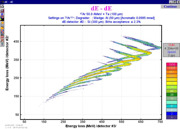
Fig.1. The example of application of a method of Monte Carlo for two-dimensional plot when the part of nucleus stops in the third detector, and the others fly by it.
To visualize two-dimensional plots on the base MC method, User has to
choose a plot of interest as it was in previous version. After standard
two-dimensional plot on the base ellipses drawing is appeared it necessary
to click on the button ![]() in the left-top corner of the plot window. To stop a acquisition, the user
should press the button
in the left-top corner of the plot window. To stop a acquisition, the user
should press the button ![]() the left key of a mouse. Accordingly to continue an acquisition it is necessary
to press the button
the left key of a mouse. Accordingly to continue an acquisition it is necessary
to press the button ![]() .
In an acquisition mode of a set the user may change a direction of the
X-axis, swap horizontal and vertical axes, make zoom or on the contrary
restore original parameters a graphics, to print out the plot and to place
or remove identification of nuclei. The method of Monte Carlo may be used
for all two-dimensional plots which have been built - in the program, such
as which example represented in figure 2.
.
In an acquisition mode of a set the user may change a direction of the
X-axis, swap horizontal and vertical axes, make zoom or on the contrary
restore original parameters a graphics, to print out the plot and to place
or remove identification of nuclei. The method of Monte Carlo may be used
for all two-dimensional plots which have been built - in the program, such
as which example represented in figure 2.
The data represented on a graphics by various color on quantity of events on the given point a graphics. The program automatically calculates a logarithmic scale with normalization for a maximum output. The given logarithmic scale of colors represented the a graphics.
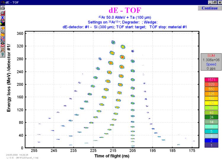
Fig.2. A Monte Carlo method for dE-TOF plot.
1.1. Speed of Monte Carlo acquisition 
During a MC data acquisition the window occurs in which the sum of the typed events and speed of a set (events per one second) is shown. Speed of an acquisition depends first of all on computer speed, and also from installations by the user for MC-method. So for example, Pentium-II (frequency 233 MHz) at standard installations of a method of Monte Carlo allows to reach speed of an acquisition up to 15 thousand events in one second that is much higher, than sometimes presume to itself of physics during experiment with registration of all events.
1.2. Settings of Monte Carlo method for two-dimensional plots
The user may make all customizations of MC-method necessary in the dialogue "Plot Options" (see fig.3). Red circles mark customizations used only for MC-method, blue squares mark items used for all two-dimensional diagrams, and by green triangles accordingly items used by default for all calculations in the program.
1.2.1. Distribution compression for Monte Carlo plot
Distributions used in the program (see the chapter 3.2. Dimension of distributions) may be compressed, for this purpose increase speed of calculations and first of all size of occupied RAM. At a plenty of nucleus and at small compression of allocations at shortage of the RAM may even be involved swapping on the disk, that appreciably will slow down operation. However strong compression of allocations worsens quality of simulation. It is necessary to find the compromise as always in similar cases. Value of compression is by default equal to 4.
1.2.2. Pixel for one event for Monte Carlo plot
All of a graphics in the program are output in virtual coordinates by dimension 1000´ 1000. To draw MC-method in colors, it is necessary to save in memory the typed data as the appropriate array who also is used for the subsequent upgrade of the screen and printing of plots. Simple counts show, that at output at permission one pixel on one unit from the array it is necessary to reserve memory hardly less than two megabytes. Certainly decrease of permission does not improve the diagram, however allows to save the RAM seriously. Recommended permission 3´ 3.
1.2.3. Resolutions and thickness defects
All resolution settings are used only for two-dimensional plots. Material thickness defect are applied also to calculate energy and range distributions for one-dimensional plots. Default values of thickness defect and energy and time resolution User may input necessary in the dialogue "Plot Options". For the next start of the code "LISE" these defaults values will be used. For changes of thickness defects of and energetic and time resolutions in calculations the user should use accordingly dialogues of materials. All defaults values are saved in file lise.ini.
It is necessary to mark, that defect of width of a material also is applied and in calculations of transmission with degrader (wedge) in the intermediate disperse focal plane where the contribution of it may be rather noticeable in transmission of fragments.
2. In-built cubic spline procedure (version 4.4)
In the previous versions for definition of a distribution value in a point x two were used simple interpolation methods: a method of a trapeze on the basis of two next with x points and a method on the basis of three points. However with introduction in the program of a new class of distributions connected to transformation of one distribution (for example on magnetic rigidity) in the appropriate distribution but already on energy the new method of interpolation cubic spline was One of advantages of a new method is the opportunity of calculation of the first and second derivatives for any point of distribution. We shall remind, that it is connected to a continuity of derivatives as cubic spline is under construction on the basis of equality of the first and second derivatives for known points of distribution:
![]() .
.
2.1. Transformation of distributions
![]()
Fig.4. The scheme of conversion of one distribution in another
In a basis of conversion of one distribution in another (the scheme represented in Fig.4) lays saving of squares between every each i-1 and i points. In the last versions the given task was solved rather simple way that had an effect for quality of conversions at such small dimension of distributions (NP=128).
The edge effects were especially appeared in distributions of energy, ranges in matter as they may not be negative. We shall assume that the nucleus with the certain distribution passes through substance and the i-point of distribution stops in matter, and following passes. Then function appropriate between i-1 and i pointspoints for preservation of the area should aspires to infinity. Rather complex mechanism of smoothing was applied. But all the same it is ideal to solve this problem it was not possible!
In the last versions the area between points was determined by the next primitive expression:
We may use now correct calculation of area is next:
 ,
,
because we have infinite function f(x) due to introduction of procedure
cubic spline.
The condition of equality of the areas in both distributions between
in an interval can be presented in the following kind:
 .
.
Doing substitution y=EB(x) it possible to get simple and good solution with application of the first derivative of the function f(x):
 .
.
This derivative can be taken with the help of cubic spline procedure having constructed distribution x from y. Using further cubic spline procedure for f (y) distribution can be proceeded from complicated distribution with a variable step between points to more simple with a constant step accordingly.
2.2. Edges effects
Introduction of new transformation of distributions yet does not solve a problem of edge effects. To resolve the given problem in the program use negative values of energy, magnetic rigidity and range in material was entered. The user certainly as always deals only with positive these sizes. The second, that was made for avoidance of edge effects in case of calculation of range in detectors (as energy loss calculation) - transformation of complicated distribution (with a variable step between points of distribution) to simple (a constant step) with positive values occurs only once for required distribution. All this qualitatively allows to expect in a case the attitude(relation) of fragments stopped in different detectors. The contribution of distribution broadening due to straggling (and also thickness defect of detectors) conducts down to the detector of interest, where already after transformation to simple distribution (with constant step between points) there is a convolution with transformed straggling distribution.
3.1 Different methods to draw one-dimensional plots
Fig.5. The dialogue "One-dimensional .plot drawing methods"
3.2. Dimension of distributions
Calculation of fragment transmission is based on an estimation of a part of distribution (spatial, angular, momentum) through given device acceptances. Under operating system DOS in old versions the dimension of distributions was equal to 64. With adaptation of the program under operating system Windows dimension became equal to 128. The increase of dimension conducts to better results, but slows down calculations and demands the greater operative memory. Especially strongly it is shown at calculation of fragments outputs with the established option of charge state condition calculation. At the same time at calculations of optimum thickness of target a step-type behaviour of calculations at small dimension of distributions becomes more appreciable. In the new version of the program the user itself may establish in dialogue "Preferences" (Fig.6) desirable dimension both for calculations without charge state condition, and with charge state condition. By default dimension of distributions is equal 128 for an option of calculation without chargt state condition, and 64 accordingly without charge state condition. In a state line of the program (Fig.7) the user always may observe the current value of dimension of distributions (NP).
Fig.6. The dialogue «Preferences»: setting
of distribution dimension.
Fig.7. The fragment of the code state line (gadget)
where it is possible to observe the current dimension
of distributions.
3.3. New plots
In the new version opportunities to compare different methods of energy
loss calculations have appeared, quickly to estimate values of range and
energy losses in material (applying ZOOM) on the basis of new plots "Plot
of Fragment Range in Target versus Energy" and "Plot
of Fragment Energy Loss (dE/dx) in Target versus Energy" which
settle down in menu Utilities.
3.4. Mode "auto" for the Wien filter and D6-dipole calculations
The previous versions automatically calculated adjustments of the Wien filter and the D6-dipole, well as showed experience sometimes it is necessary to have possibility to disable this mode to put any values. In the new version the given possibility has appeared. The user may in appropriate dialogues of adjustment of the filter and the dipole to place or remove an option "automatically". If this option is placed, the flag will appear in the window of adjustments (see Fig.8). It shows that calculations of parameters of the Wien filter and dipole D6 occurs automatically to changes of the setting fragment and magnetic rigidity of the second dipole.
3.5. Note of base configuration used for calculations
At start of the program the configuration of the LISE3 spectrometer boots. The user may load other configuration files or create the new configuration file. Fast to find out with what configuration he works (instead of to look at an example optical coefficients) in standard program files with extension "*.liz" and in files results "*.res" the name of the base configuration is saved.
3.6. Bugs
3.6.1. Energy loss calculation in thin material
In the previous versions of the program at calculation of the residual energy after passage by a nucleus of a material with thickness close to 0 user may receive, that the residual energy exceeds initial! Calculation was carried out as follows: initial energy Ei was transformed through tables to range Ri, then detector thickness t was subtracted from Ri and already received value Rr was taken away was transformed to energy Er. In the new version for avoidance of this effect the following amendment is entered: the range Ri is again translated in energy Ei*, and then the difference (Ei*- Er) is subtracted from initial value of energy Ei to get final residual energy Er*.
3.6.2. Calculations with a primary beam in dialogues TOOLS and Physical calculator
The bug of calculations with a primary beam in dialogues "TOOLS" and "Physical calculator" was found out. It was corrected.
4. Brief description of previous version (4.2.1-4.3.15) changes
version 4.3
1. Two possibility to calculate angular transmission (Dialog "Acceptances")
2. The M5678-spectrometer(at Dubna) plot has been added
3. Pictures in the dialogs "Curved degrader" & "Angle on the target" has been corrected.
4. The Bug in the dialog "Beam" (the button "Table of Nuclides" didn't work) has been corrected.
5. Calibrations of all LISE's magnets have been added (see Fig.9).
6. Calibrations of setting of the angle on the LISEs target have been corrected.

Fig.9. Plan of the LISE spectrometer with buttons of calibrations dialogues of spectrometer elements.
version 4.2.5
Calculation of material thickness between start energy and energy rest has been added in the Physical Calculator (see Fig.10).
Fig.10. The dialogue "Physical calculator": new possibility to calculate of material thickness between start energy and energy rest.
version 4.2.4
Utilities -> LISE3's calibration (dipoles, Wien-filter): Transformation between values of Brho, B real(affiche), B red(lu), I(Ampere) for the LISE dipoles D3.DP1(D3) and D3.DP2(D4).
version 4.2.3
Utilities -> Curved degrader: Calculation (see Fig.11) and plots (see Fig.12) of curved degrader profiles for different operating modes (achromatic, monochromatic, homogeneous).
Fig.11. The dialogue "Calculation of curved degrader in the IDPF".
Fig.12. The plot "Curved degrader in the IDPF".
version 4.2.2
Utilities -> Calculation of angle on the LISE target: calculation
magnetic fields (also dipoles currents ) of two dipoles to get the determined
angle on the target (see Fig.6).
Fig.6. The dialogue "Calculation of angle on the LISE3 target calculation magnetic fields (also dipoles currents ) of two dipoles to get the determined angle on the target.
version 4.2.1
Energy distribution plot after wedge has been corrected.
5. Next steps of the code development