|
THE CODE
LISE++: version 6.1 Block
structure: design your own spectrometer
|
|
Contents: 1.3. Support of
“classic” LISE files 2. Design your own spectrometer 2.1. Set-up
dialog: new main feature 2.2.1. Settings of spectrometer scheme 3. Description of Blocks and their properties 3.1.1. Optical block: properties and methods 3.1.1.1. Optical
matrix of LISE++ block 3.1.1.2.
Acceptances and slits 3.1.1.3.
Momentum acceptance of spectrometer 3.1.2. Blocks from optical class 3.2.2.1.
Computational values (fields) 3.2.2. Dispersive block on the base of Magnetic dipole 3.2.4. Compensating dipole after the Wien velocity filter 3.3.1. Material (detector) block: properties and methods 3.4. Degrader in
the dispersive focal plane 3.4.1. Wedge angle calculation 3.4.2. Possible problems in wedge angle calculation 3.4.5. Double acceptance effect 4. Transmission and fragment output calculations 4.1.
Transmission calculation in a block 4.1.1. Transmission statistics 4.4. Previous
isotope area rectangle 5. Improved mass formula with shell crossing corrections. 5.1. Shell
crossing corrections 5.2. Use of LDM
parameterizations in LISE++ 5.3. LDM
parameterizations and accuracy of cross-section calculations 6.4. Dialogs
Goodies & Physical calculator 6.6. Range
optimizer – Gas cell utility 6.8. Cyrillic
and Hex-style converter 8. Future developments of LISE++ 1. IntroductionLISE++ is the new generation of the LISE code, which allows the creation of a spectrometer through the use of different “blocks”. A “block” can be a dipole (dispersive block), a material (i.e. a given thickness for a detector), a piece of beampipe, etc. The original LISE was restricted to a configuration consisting of two dipoles, a wedge, and a velocity filter. The number of blocks used to create a spectrometer in LISE++ is limited by operating memory of your PC and your imagination. The code has an improved interface, new utilities were added, and the spectrometer scheme in the program allows quick editing of blocks. 1.1. How to download LISE++As with LISE, LISE++ is distributed freely and is accessible through ftp-servers in East Lansing (http"//lise.nscl.msu.edu/download) and Dubna (ftp://http:"//lise.nscl.msu.edu/). Dubna ftp-server does not support Netscape. Contents of the LISE ftp site and detailed information about downloadable files can be found in http"//lise.nscl.msu.edu/downloadreadme. The new version LISE++ should be installed in the previous LISE directory as to not duplicate certain files (for example the mass database). The previous version will still work if this is done. G If
you have already installed one of LISE++ (6.0.**) beta versions, it is
strongly recommended to reinstall it with the newest version. 1.2. New file formatsThe LISE++ program has a new file format for all of the files it uses and creates. The extensions of these files were changed to avoid overlap with files of the LISE program. Three new types of files were added: a file containing a profile of a curved degrader, a file containing calibrations of dispersive optical blocks, and a matrix file. The new extensions are given in Table 1. Table 1. File extensions used by LISE and LISE++.
Note: The regular LISE++ file (extension
"lpp") consists of the Configuration file (lcn), the some sections
of the Option file (lopt), the experiment settings and calculation results: LPP = LCN + LOPT + Experiment settings +
Calculation results File names of calibration and degrader files are saved in the configuration file. Note: Upon
starting, the code reads the LISE.INI file which contains the default
configuration and options file names, as well as the list of most recent
files. The code loads the default configuration file and the default options
files. If these files are absent the user is informed and the standard LISE
settings are used. The user can set the default configuration and option
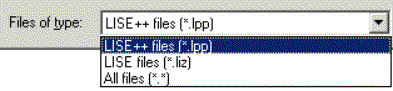
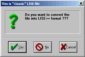
files in the dialog "Preferences". 1.3. Support of “classic” LISE filesLISE++ can read all old-format files (regular, configuration, option), but it only saves just in its own format. If you choose old-format files (for example “liz” instead “lpp”) the code will propose to recalculate transmissions of fragments and then ask if you want to save this file in the LISE++ format.
G If you used a LISE++
(6.0.**) beta version, and the configuration files A1900-4dipoles.lcn and
A1900-2dipoles.lcn are found in the directory “<LISE>\config”, then it
is necessary to delete them. Corrected A1900’s configuration files are found
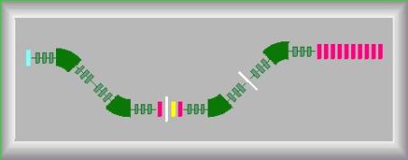
in the directory “<LISE>\config\NSCL”. 2. Design your own spectrometerThe “classic” LISE code uses only one configuration of a spectrometer consisting of two dipoles: LISE “classic”: Target + Stripper Þ Dipole1 Þ Wedge Þ Dipole2 Þ Velocity Filter Þ 7 materials LISE++ block â
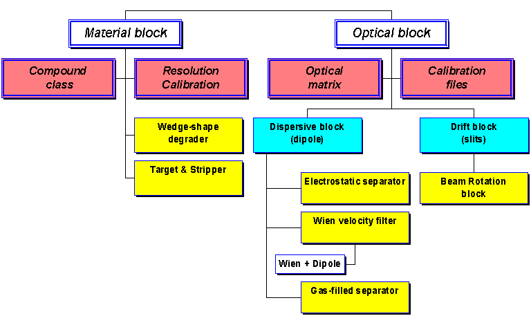
Fig.1. LISE++ block hierarchy There were a lot requests from users to increase a number of materials, to put a velocity filter in beginning of a spectrometer, to put additional materials between dipoles, etc. All this is now possible in LISE++. The user can choose and place blocks in the spectrometer at own their discretion. The main class “BLOCK” in the program is inherited by classes “Material” and “Optical” (see Fig.1). The basic properties and methods of these two classes will be considered in this chapter. Currently, LISE++ has eight blocks and three more block are under development (Table 2).
2.1. Set-up dialog: new main feature
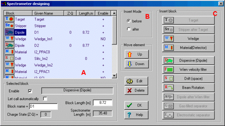
Pressing on the button “Setup” in the toolbar (or through the menu “Settings Þ Spectrometer designing”) brings up a dialog “Spectrometer designing” (Fig.2) and allows you to begin designing a fragment separator. This is the main new feature of LISE++. The first two positions are occupied by the blocks “Target” and “Stripper”. There are fixed, it is impossible to delete or move them. Insert a new block: · In the column “Block” of the window (“A” in Fig.2 - Spectrometer window) click on an existing block, which you want to insert a new block before or after; · Choose an insert method “before” or “after” (“B” in Fig.2), · In the frame “Insert block” (“C” in Fig.2) click on the icon of the block you wish to insert. Delete block: · Select a block you want to delete in the Spectrometer window, ·
Press on the button Move block: · Select a block you want to move in the Spectrometer window, · Press on a button “Up” or “Down” in the frame “Move element”. Edit block: · Select a block you want to edit in the Spectrometer window, ·
Press on the button or · Double click, using the left mouse button, on the block you want to edit in the Spectrometer window.
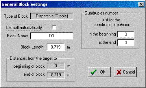
Fig.2. The dialog “Spectrometer designing” is the first step designing fragment separator. It is possible to edit some properties of the selected block in the frame “Selected block” in the bottom left corner of the dialog. Checkbox “Enable”: all new blocks are available automatically. It is impossible to disable the blocks “Target” and “Stripper”. If a block is set to disable, then this block is not shown in the Setup window and in the spectrometer scheme and the message “NO” will appear opposite this block in the column “Enable” of Spectrometer window of the dialog. A disabled block is not taken into account in transmission and spectrometer optic calculations. G It is
possible to change mode (“enable / disable”) of a block only in the dialog “Spectrometer
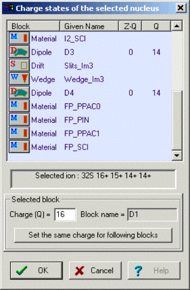
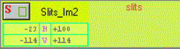
designing”. Checkbox “Let call automatically”: · On: the block name is called automatically using the name of the block type and its order number in the spectrometer; · Off: the block name may be entered manually. It is desired to input short names (less than 10 characters) to avoid a name truncation in the Setup window; · All new blocks are called automatically. Block name: The name of the block appears in all dialogs and menus connected with this block. If the option “Let call automatically” is set “Off”, then the user can input a new name for the block. It is recommended to name the block so that it is clear from the name where the block is located. For example the name “Slits_Im2” is used to describe a drift block in the mode “slits” found in the location “Image2”. Block length: the code uses a material block with zero length for the spectrometer length and time-of-flight calculations. Just optical blocks may have a length to determinate a spectrometer length and calculate time-of-flight. More on the length of optical blocks will be mentioned later in more detail. Charge State (Z-Q): if the option “Charge states” (in the dialog “Preferences”) is set, and this is an optical dispersive block, then the cell “Charge state” is enabled and you can edit the charge state value for the setting fragment. More details about charge state calculations and their transmission is found in chapter 4.2. G All operations in the
dialog will be carried out without an opportunity to restore a former
configuration. In other words the operation UNDO does not work in this
dialogue. All changes will be shown in the “Setup window” of the code and in
the spectrometer scheme only after leaving this dialogue. 2.2. Scheme of spectrometer
The user must be careful to set the correct length of dispersive
block, which includes the quadruples and dipole(s). The dispersive block
length should be always more than the dipole length, equal to the product of the
radius of the dipole(s) and the angle (in radians). The difference between
these lengths is the total length of the quadruples in that block. ·
The user can select a
block on the spectrometer scheme by moving the mouse over it (turning the
block dark blue), thus selecting it and allowing the user to click on it to
bring up a dialog. ·
To Edit block
properties: click on the selected block once using the left mouse button. ·
To Edit block
acceptances and slits: click on the selected block once using the right mouse
button. ·
Drift blocks in the mode
“Slits” (block length is equal to 0) is shown by thin long line perpendicular
to the beam axis. In other words the length of the drawn block is
proportional to its real length. ·
Materials with zero thickness
are not shown in the scheme.
3. Description of Blocks and their properties3.1. Optical blockThe hierarchy of optical blocks is shown in Table 3. Table 3. The hierarchy of optical blocks.
The description
of classes is explained in the text. First the methods used in a class will be
described for each class, then blocks used for constructing the spectrometer
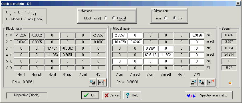
on the basis of a given class will be explained. 3.1.1. Optical block: properties and methods3.1.1.1. Optical matrix of LISE++ blockThe “Optical matrix” class is based on a class “matrix” of constant, 6´6, dimension and has the capability of transforming matrix elements of different units (mm Û cm). LISE++ has two optical matrices for each optical block: “global “and “local”. The local matrix belongs just to one block and does not depend on other blocks. The program keeps all local matrices in configuration files. This is so the insert/removal of a new block in/from a spectrometer does not change the matrices of other blocks. The global matrix of the block is computed on the basis of ALL the previous blocks and the local matrix of this block. It is possible to present i global matrix calculations as recursive equation: Gi = Li ´ Gi-1 , Where G is the global matrix, and L is the local matrix. The global matrix of the first optical block is equal to its local matrix. The program uses elements from both matrices in fragment transmission calculations. The code automatically recalculates all global matrices if one of local matrices changed. Clicking the button
Fig.6. The “Optical matrix” dialog. In the LISE “classic” version the user could only edit local matrices. LISE++ not only allows you to edit local and global matrices by element as described above, but also allows to you input entire matrices using matrix files. Inserting matrices into the program LISE++ from the program TRANSPORT [Bro80] can be done using the following steps: · Choose a matrix corresponding to the block you want to change in the TRANSPORT result file and copy it to a new file. · Save the file with extension “mat”. 6 1 -2.30374 0.00092 0.00000
0.00000 0.00000 2.88863 10.75650 -0.43836 0.00000 0.00000
0.00000 0.00011 00.00000 0.73813 0.00023
0.00000 0.00000 0.00000 00.00000 37.30313 1.36628 0.00000
0.00000 0.00000 03.10718 -0.12663 0.00000 0.00000
1.00000 -0.24222 00.00000 0.00000 0.00000
0.00000 0.00000 1.00000 Fig.7. Example
of matrix file (unit “cm”). · Create a new blank line in the file before the matrix elements. The first line of a file has to contain two numbers. The first shows matrix dimension (matrix is always supposed to be a square matrix). The second value is the dimension. 0 corresponds to “mm”, 1 corresponds to “cm”. If the second number is missed, by default it is supposed to be equal zero. The first line of the TRANSPORT matrix file should contain “6 1” (see Fig.7). The next six lines are matrix elements corresponding to the rows of the matrix. A separator between elements can be tabs, spaces, commas, or semicolons. ·
In
the “Optic matrix” dialog click on “Global” to go to the mode of global
matrix editing. Click on the button The dialogs of optical matrices depend on the block, and their features will be further explained in later sections. Reading of data in the matrix dialogs is not instantaneous, but is takes approximately 1 second in which you can see a blinking heart in the lower right corner of the dialog. v To
save a matrix in a file it is necessary to press the button v To
get an inverse matrix press the button G One way to check if the input values are corrected when
then you are editing a matrix is to calculate the determinant. The
determinant of an optical matrix should always be about 1. The determinant of
a matrix is automatically calculated and displayed in the lower left, below
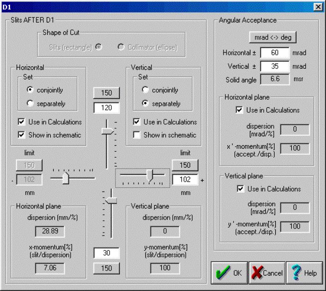
the matrix. 3.1.1.2. Acceptances and slitsIn the “classic” LISE program there was
just one dialog for all the slits and acceptances of the spectrometer. In
LISE++ each block (excluding “Rotation beam”, “ Stripper”, and “ Wedge”
blocks) has its own “Slits & Acceptance” dialog (see Fig.8), which is available by clicking in the dialog of
the optical block properties through the button
Fig.8. The “Slits & Acceptance” dialog. The editing of slit sizes is more visual and convenient in the new version, as well as the use of slits is closer to the reality of an experiment. The maximum slit size is defined by the user. In LISE++ it is not possible to input a moment acceptance that frequently resulted in fallacy earlier. The momentum acceptance is now determined by the slit size and dispersion (x/d). Also, the program can calculate a momentum acceptance from the angular dispersion (q/d) and angular acceptance and takes that into account in transmission calculations. It plays an important role in case of small dispersion (x/d) and large angular dispersion (for example: block “Slits_S800BL” in the configuration file “A1900+S800_d0.lcn”).
·
If the block has working slits then the
Slits are found AFTER the optical
block and · Angular acceptance is applied on the BEGINNING of the block 3.1.1.3. Momentum acceptance of spectrometer
G There
are specific cases when the real TMAS actually will be more than shown by the
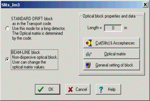
program. The “double acceptance effect” is explained in chapter 3.4.5. 3.1.2. Blocks from optical class3.1.2.1. Drift blockA drift space is a field-free region through which the beam passes. There are three types of drift block classes (see Fig.10): v Standard drift block (as in the TRANSPORT code [Bro80]): Use this mode for a finite length detector in place of a detector with zero length in the spectrometer length calculation. The optical matrix is determined by the code on the base of block length. v Beam-line block: non-dispersive optical block. User can change the optical matrix values. v Slits mode: if the block length is equal to zero without dependence from a above-mentioned mode. The optical matrix of block in this mode is unitary.
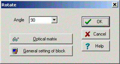
3.1.2.2. Rotation beam block
The block is used
at transitions of one plane to another. For example, the A1900 spectrometer
is in a horizontal plane, and then the beam follows the S800 beam-line which
is in a vertical plane. 3.2. Dispersive blockOptical
dispersive blocks are electromagnetic separation devices. Only Dispersive
optical blocks determine the setting of the spectrometer on a certain
fragment. 3.2.1. Properties and methods3.2.2.1. Computational values (fields)Classification of electromagnetic
separation devices (LISE++ dispersive blocks) and
their selection methods is given in Table
4. Magnetic (electrical) fields of dispersive blocks
can be calculated by the code, as well as the user can enter manually field
values. The basic difference of dispersive blocks from optical blocks is that
the adjustment of the fields of these blocks result in a change in the
trajectory of particles and therefore their separation in space. When
the spectrometer is “set” on a fragment, it means that the magnetic
(electrical) rigidity of a particle coincides with magnetic (electrical)
rigidity of electromagnetic devices in the central trajectory. The magnetic
field (for a magnetic dipole) is calculated from the magnetic rigidity of the
device using a dipole radius. If a calibration file (see the next chapter for
a definition of the calibration file) is entered, then the electric current
(I) is also taken into account. Table 4. Electromagnetic separation devices.
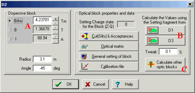
Fig.12. The “Dispersive block” dialog. You can
do the things listed below using the options in the “dispersive block” dialog
pictured in Fig.12: q You can manually change the magnetic field and the electric current using the dialog (see Fig.12 “A”). The magnetic rigidity will be changed automatically. q
You
can calculate a rigidity of the block for a given setting fragment depending
on a previous or following dispersive block values with the materials between
them taken into account (Fig.12 “B”). q You can use the rigidity value of the block to calculate the field values of all the other dispersive blocks in the spectrometer (Fig.12 “C”). q Clicking on
the button 3.2.1.2.Calibration file
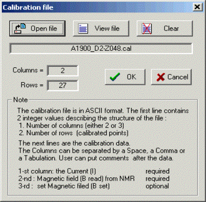
The format for the calibration file is rather simple. You can see the format description in The “Calibration file” dialog (Fig.13). The program uses a cubic spline to get a value in region indicated in the file. The code uses a linear extrapolation if the searched value exceeds the determinate region. Bread is a measured value from a electromagnetic device (for example a NMR probe). Bset is established using the calibration. The program uses the Bread value to calculate a magnetic rigidity. If just one calibration between the magnetic field and electric current is entered, then B=Bread=Bset. 3.2.2. Dispersive block on the base of Magnetic dipoleThe program uses the
definition of a “Dispersive block” instead of simply a “Magnetic dipole” to
underline that this block is a system with one optical matrix but consists of
quadruples, drifts, and magnetic dipoles. The “Dispersive block” dialog is
presented in Fig.12. The
basic characteristics and properties were described above in the text. The order of distribution and transmission
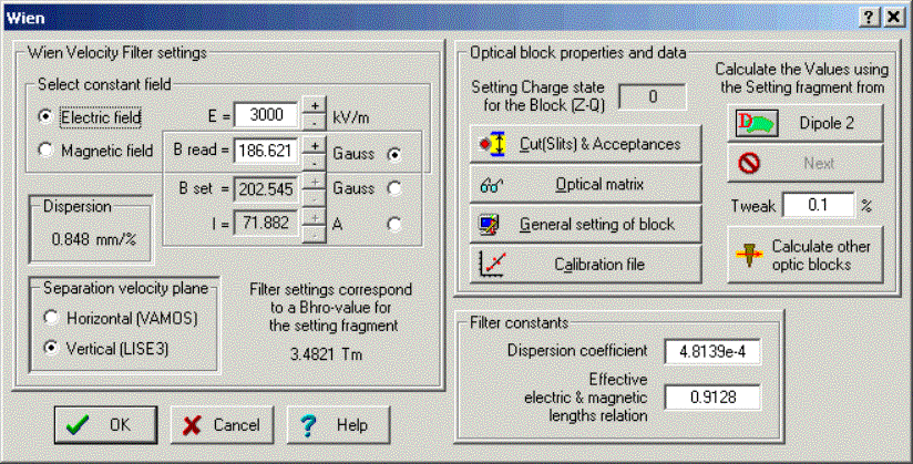
calculations in the dispersive blocks is given in chapter 4.1. 3.2.3. Wien velocity filterLISE++ assumes the velocity filter is a standard dispersive block with the optical matrix and all other properties and methods. This redefinition in comparison with the “classical” version allows the use of the filter anywhere in the spectrometer. Velocity dispersion through the filter depends on the mass and charge of a particle and is function of the particles energy. The most important difference between the filter and a magnetic dipole is that dispersive elements of the local optical matrix are recalculated for each fragment and energy anew for the Wien velocity filter. The filter operates with two fields. Therefore to adjust the filter on a one fragment, you should keep one field constant (see the frame ”Select constant field” in Fig.14) and change the other field. In a reality the electrical field is kept constant, while the magnetic field is changed.
Fig.14. The “Wien velocity filter” dialog. The LISE code has three parameters to define the filter of velocity: o eElen - Effective electric length, o eMlen - Magnetic effective length, o rrf - Real/Read field. There is just one parameter “Effective electric & magnetic length relation (EMLR)” in the LISE++ (see the frame ”Filter constants” in Fig.14), which is a combination of three of these LISE parameters using the formula: EMLR = eElen · rrf / eMlen. 3.2.4. Compensating dipole after the Wien velocity filterIt is
planned to develop a dialog for a compensating dipole after the Wien velocity filter as in LISE
(it was named dipole D6). The compensating dipole is a dispersive block
assigned to compensate the velocity dispersion after the Wien velocity
filter. Using the compensating dipole it is possible to get the A/Q dispersion.
The main advantage of A/Q selection is absence of a momentum (velocity)
dispersion which allows you to use the large momentum emittance of the secondary
beam. However, you can simulate the compensating dipole in LISE++ already
now. To do so, you have to put a dispersive block after the Wien velocity
filter and manually input a dispersion of the block to compensate the filter
dispersion, such that after the compensating block the global dispersion is
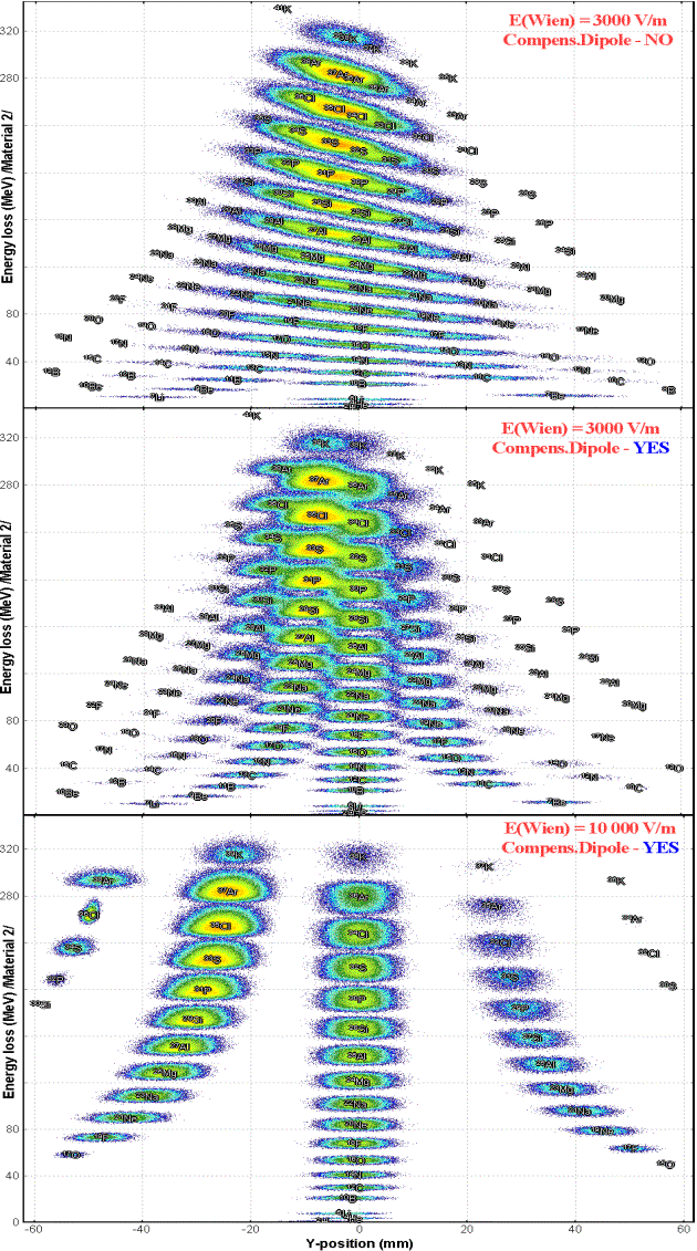
equal to zero. Fig.15 shows selections by the system “velocity filter Ä
dipole” for different values of the electric filed of the velocity filter. This example
is accessible through the LISE web-site: http://lise.nscl.msu.edu/6_1/examples/lise_wien_d6.lpp 3.3. Material blocksMaterial blocks were created on the basis of the LISE++ Block class and the LISE Compound class. There are four existing blocks (Target, Stripper, Material, Wedge) and one (Secondary target) still under development. Material blocks properties are given in Table 5. Table 5. Properties of Material blocks.
New dimensions (mm and g/cm2) were added in LISE++ to
avoid it excess characters. The user can choose system of
measurement units in the frame “Dimensions” of the “Material block” dialog
(see Fig.16). Material (detector) and Target blocks own the optical blocks property: Slits. To correspond to a reality, the supports of a material act as slits and therefore are ahead of the block. The slits used in the program have the rectangular form. Use of oval slits is planned in the future.
The calculations will be made using the values
of the Dispersive block before the material with the new thickness of this
material taken into account. The material block is not shown in the
spectrometer scheme if the material thickness is equal to zero. In the Set-up
window a blank space is shown instead of zero. 3.3.1. Material (detector) block: properties and methods
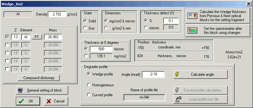
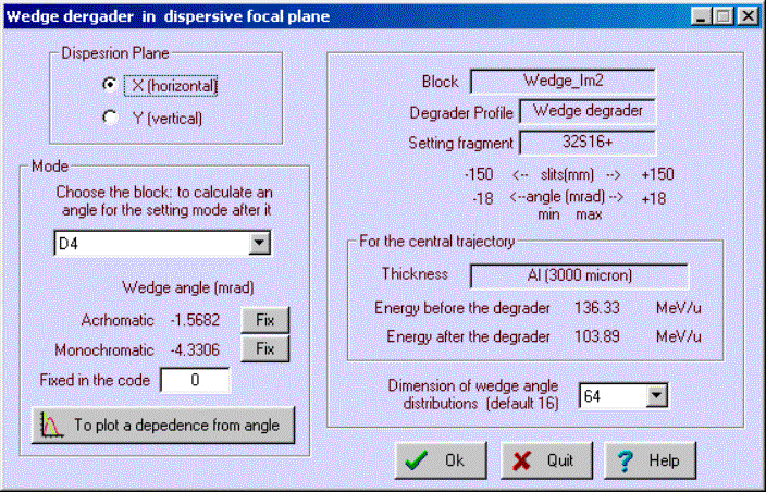
3.4. Degrader in the dispersive focal planeLISE++ supports three types of degrader profiles: wedge profile, homogeneous (a simple material), and curved profile. To calculate a wedge angle or a curved profile, the code uses the modes: achromatic and monochromatic. Also you can enter an angle manually, or have the code calculate a wedge angle for you (see the frame “Degrader profile” in Fig.18).
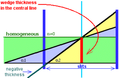
Fig.18. The “Wedge (Degrader in the dispersive focal plane)” dialog. Coordinate (X) in the frame “Position-thickness” is defined as smallest slit between the previous and next dispersive blocks. These coordinates determinate maximal possible angle of wedge: Angle limit = arctan ( Thickness central trajectory [mm] / Slit [mm] / 2 ) (see Fig.19). G The
angle of the wedge is not recalculated automatically as in the classical
version. The angle of the wedge or the curved profile are always kept such
that they correspond to the reality of an experiment.
3.4.1. Wedge angle calculationLISE++ can calculate a wedge angle from the conditions that the wedge must be achromatic or monochromatic after the block defined by the user. In the classical version the wedge is found between two dipoles and the angle is calculated for the focal plane after the second dipole. In LISE++ a wedge can be placed in anywhere. It is necessary in the frame “Mode” to choose the block after which conditions will be applied. If you press one of the keys “Fix” or enter a value into “Fixed in the code” cell manually (Fig.20) than the program uses one of calculated angles in the further calculations.
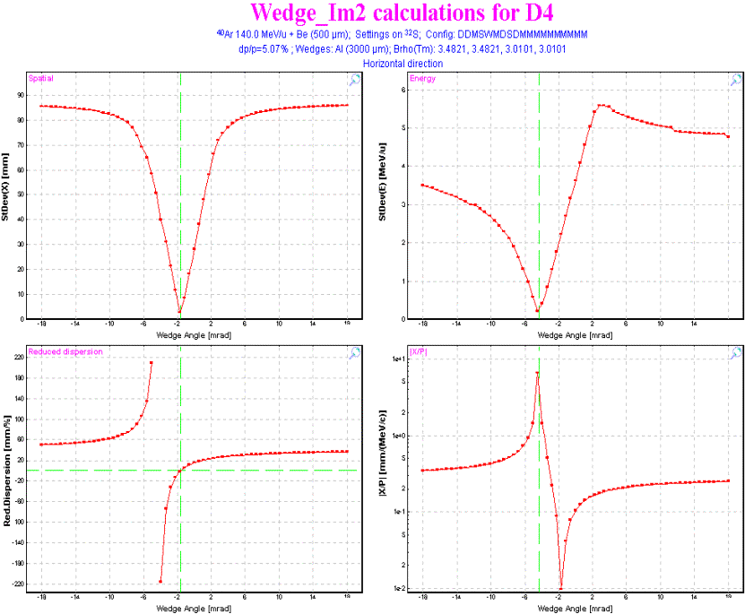
Fig.20. The wedge angle calculation dialog. LISE++ calculates the wedge angle when this dialog is loading or when one of the parameters (block, number of points in distribution) changed. The code determinates the minimal (amin) and maximal (amax) values of angle (as well as Angle limit from the previous section). The program N+1 times calculates a setting fragment transmission changing a wedge angle for the value (amax - amin) / N. As a result of these calculations the program fills four distributions which can be plotted by clicking “to plot a dependence from angle” in the frame “Mode”. The received wedge angular distributions are shown in Fig.21. A description the wedge angular distribution is shown in Table 6. Table 6. Wedge angular distributions.
Fig.21. Wedge angular
distributions. The code seeks minimums in spatial and energetic distributions. The code defines angles using neighboring points of these minimal points by a simple expression. To get more precise wedge angles, it is necessary to increase the number of points in the wedge angular distributions. A default value of the distribution dimension is defined in the dialog “Preferences”. Press the key “Escape” once if you want to break calculations. If the code didn’t find a solution for one of a mode or you interrupted then you will see a string “???” instead of a calculated angle value. Button “To plot a dependence from angle” will be inaccessible if · Calculations were interrupted · The transmission of the setting fragment after chosen block is equal to zero for all points of the wedge angular distributions. 3.4.2. Possible problems in wedge angle calculationWorking
with the beta-version many users had questions and problems with wedge angle
calculations. On the basis of their remarks, the program was modified to display
messages indicating why a wedge angle was not is calculated. See Table
7 for messages problems, reasons then to correct the
problem. Table 7. Possible problems in wedge angle calculation and methods of their elimination.
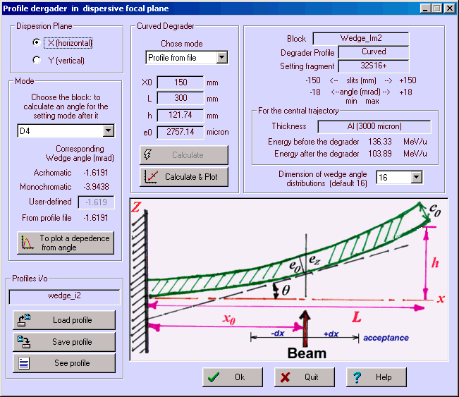
3.4.3. Curve profile degraderLISE ++ has a new profile of degrader that can be used for transmission calculations: a curved profile degrader. If in the classical version only a wedge shape degrader was applied to transmission calculations, but in the new version a curved profile degrader also can be applied for transmission calculations.
· By analogy to
the “Wedge angle calculation” dialog (Fig.20), the user should select a block and mode. · It is
necessary to define support parameters X
and L. A degrader length should
be approximately the slits size. · Pressing on
the button “Calculate & Plot”, the program will calculate a support of
curved degrader. · Save the
calculated profile in a file. The user can load already created structures from a disk. The parameters of a support from a file will be shown in the dialog and can be visualized in the plot. It is possible to see the corresponding wedge angle from profile file in the dialog. This angle is calculated on the basis of the support and a material used at this moment in the wedge block. The files of supports have the extension “degra” and are by default in the directory “\degrader”. 3.4.4. Use
of two wedges
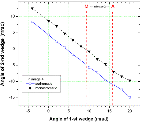
The new version has the opportunity to use multiple wedges at once. Examples of ways to use two wedges are: 1. Select an isotope of interest using an achromatic wedge to partially eliminate impurities. Then use a monochromatic wedge to get a monoenergetic secondary beam without impurities at the end of spectrometer. 2. To eliminate (by the second wedge) products of secondary reactions from the first wedge. This is very useful for particles at relativistic energies. 3. To increase the spectrometer momentum acceptance (see the next chapter).
In this configuration wedge angles can be written by: Achromatic mode in Image4 a1 + a2 @5 mrad, Monochromatic mode in Image4 a1 + a2 @ 10 mrad. 3.4.5. Double acceptance effectThe use of two wedges can
result in an effect, which we have named the “double acceptance effect”. The
“A1900-4dipoles” configuration is used. The calculated momentum acceptances
in Image1, Image2, and Image 3 are equal to 5.07%, 10.39 %, and 5.07%
respectively. Therefore, the momentum acceptance of the spectrometer is equal
to 5.07%, which the user can see in the Information window. Let’s consider
the reaction 36S(140MeV/u, 100pna)+Be(1g/cm2) with 30Ne
as the setting fragment. 30Ne’s rate at the end of the spectrometer
is equal to 3.3e+1 pps, and only 54 % of all fragments pass through
the slits in Image2. Now let’s put a wedge (Be, 0.7g/cm2) in Image1 and choose the angle of the
wedge (22.5mrad) which is the maximum possible from the slits. The wedge is
not achromatic; it works as a lens focusing on Image2. 30Ne’s
rate at the end of the spectrometer is equal to 5.6e+1 pps, and 98% transmission through the slits in
Image2. Now the momentum
acceptance of the spectrometer is determined by
the slits in Image1, instead of by the slits in Image2, and therefore the
rate has doubled. If a degrader is put in Image 3 that is identical to the wedge in Image1 and an angle is calculated to be achromatic for Image4 (angle = -14 mrad), it is possible to select 30Ne from the impurities which comprise about 65% of the beam. Calculation results for configurations with different numbers of wedges are shown in Table 8. From this table it follows that the best selection is reached when the wedge is found in a plane with maximal dispersion. But in this case the rate is lower, but the quality of a secondary beam (emittance, purification) is much better, than in the case of the use of two wedges. As always there is the balance between quantity and quality. Table 8. Calculation results for configurations with different numbers of wedges.
The LISE++ files
with these calculations are accessible through the LISE web-site: http://lise.nscl.msu.edu/6_1/examples/double_acceptance_1wedge.lpp 4. Transmission and fragment output calculations
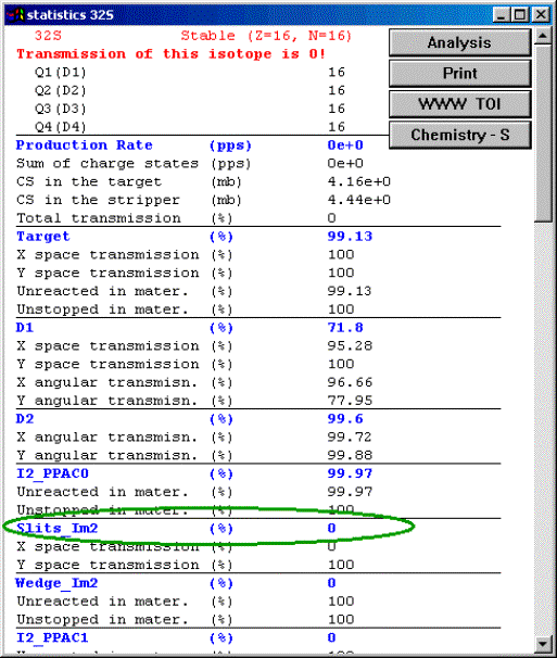
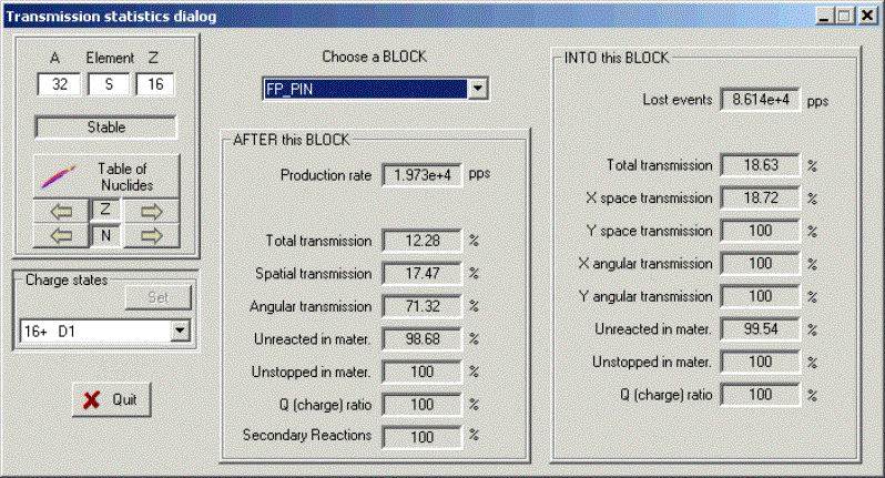
G If a telescope, with certain slits in front of it,
is placed in the end of the spectrometer, losses on the slits will not enter in
the total transmission value. For example, FP_PIN detector after dipole 4 has
its own slits of ± 25 mm in the configuration A1900-4dipoles. But
the dipole D4 slits are equal to ± 150 mm. A loss of rate on FP_PIN
slits is expected, but it will be not incorporated to the total transmission
value. G Let’s suggest a scenario in which all secondary
particles are stopped a telescope in the end of the spectrometer. If an
optical block is put after the telescope then transmission of all particles
will be equal to 0, and the code suggests no events were transmitted through
the spectrometer. 4.1. Transmission calculation in a blockThe orders of
distribution transformation and transmission calculations in the dispersive
and material blocks are given in Table
9. Table 9. Transmission calculation order in block.
Fig.26. The transmission analysis dialog. 4.2. Charge states
The default value of the transmission distribution dimension in the charge state mode has been decreased to a value of 32 in comparison with the “classical” version (64). This is to facilitate more complicated transmission calculations. It is possible to change this value in the dialog “Preferences”. 4.3. Results fileIn connection with global reconstruction of the program, the result file also has undergone a number of serious changes. As before, the user can create, look and print a result file through the menu “File Þ Results”. The file will be saved with the same name as the name of the LISE++ file in the same directory, but with the extension “res”. The result file contains calculations of energy losses and times of flight along with standard deviations. The same subroutine used to create the result file is used to calculate values (using the resolution of detectors) in the dialog “Goodies” and in the ellipse mode of two-dimensional plots. Structure of the result file is: ·
Header: brief spectrometer configuration
and basic options, · Table 0: Transmission and Rate calculations, · Table 1. Time of flight, Energy after stripper, · Table 2. Energy after blocks, · Table 3. Energy loss in materials. G Be
careful when printing a result file. The width of the page depends
proportionally on the quantity of blocks in the spectrometer. Print in
landscape mode instead of portrait, or use a word-processor to prepare the
file for printing. 4.4. Previous isotope area rectangleIt is possible
just once to choose a rectangle of isotopes of interest to calculate their
transmission by the button “Calculate area of nuclei” 5. Improved mass formula with shell crossing corrections.Accurate predictions of the production cross-sections of rare isotopes are important in the study of astrophysical processes and in the location of drip-lines. Reaction models as the abrasion-ablation, statistical multifragmentation or fusion-evaporation models rely on parameterization of the nuclear masses. This may lead to large inaccuracies in the case of discrepancies between mass parameterization and the experimental masses. Representation of nuclei as liquid drops has been very successful in predicting their properties and masses, especially those along the valley of stability. However, a large discrepancy is observed for the classical Liquid Drop Mass formula and experimental values due to the shell structure. LISE++ uses a new mass formula with shell crossing corrections. The most commonly used Liquid Drop Mass (LDM) formula (first developed by Von Weizsaecker) is where the nucleus binding energy is presented by sum of the terms shown in the table below:
Where Z and A are the charge and mass number; aV, aS, aC, aSym, d are coefficients; delta is equal to +d for Z and N are even, and -d for Z and N are odd, and zero for A is odd. Let’s name this formula by LDM0. Meyers and
Swiatecki [Mye66] have generalized this expression for the more general case
of distorted nuclei:
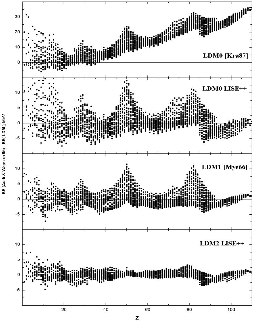
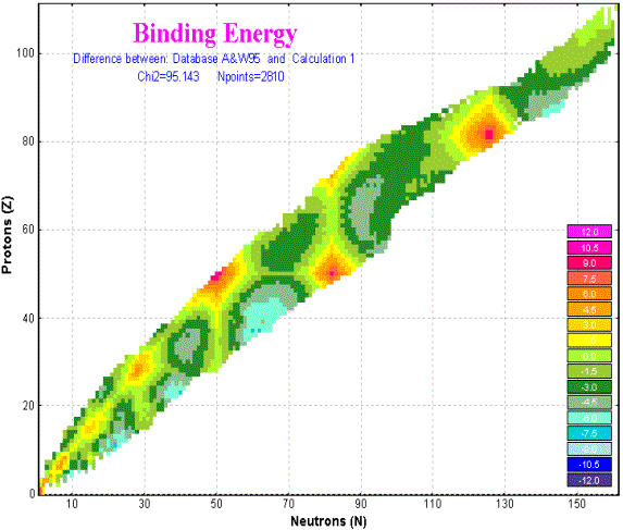
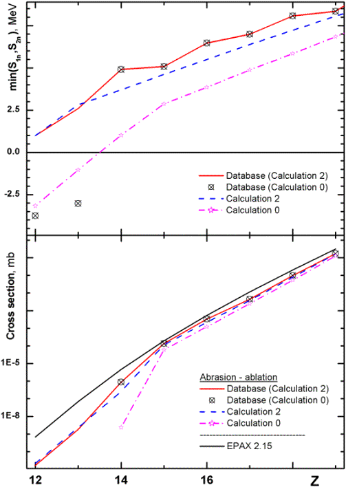
Where x is ((A-2Z)/A)2 ; aSx, aVx, aCx are the coefficients; the term Symmetry is equal to 0 in this formula, aSx and aVx suggested to be equal. Let’s name this formula by LDM1. The formula LDM2 represents the formula LDM1 with shell crossing corrections, which are described in the next chapter. Table 10 shows parameters for all these models including a new fit of parameters using the LDM0 formula (LDM0 LISE++). Fig.29 shows differences between binding energies from experimental masses [Aud95] and different LDM parameterizations. Table 10. Parameters of different LDM parameterizations and their c2 with experimentally deduced binding energies (2810 recommended values [Aud95] have been used).
Fig.29. Differences between binding energies from experimental masses [Aud95] and different LDM parameterizations. 5.1. Shell crossing corrections
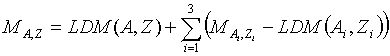
5.2. Use of LDM parameterizations in LISE++The parameterizations LDM0 (LISE++), LDM1 and LDM2 are used in the code and named correspondingly Calculation 0, Calculation 1, and Calculation 2. Mass calculations are used: ·
To
extrapolate mass of nuclei absent in the inbuilt database. These masses are
kept in the operating memory and used for calculations every time the code
needs an isotope mass. The extrapolated
mass of a nucleus is equal to:
where the nuclei (Ai,Zi) are the closest known nuclei ,in the database, to the unknown nuclei of interest. · To calculate widths of different channels of particle emissions in the Abrasion-Ablation or “LisFus” models if option “for separation energies use” is set to “semiempirical formula” in the “Setting of Prefragment and Evaporation calculations” dialog. In the ”Production mechanism”
dialog it is possible to choose one of LDM parameterizations in order to use
it in calculations mentioned above. From the “Database” dialog it is possible
to load the “Calculations” dialog (Fig.31), which with the user can see isotope characteristics
calculated by various models. Using the “Database” dialog and LDM models plot
options (Fig.32), the user can construct not only different model
distributions, but also differences between distributions of various models
(see for example Fig.30). 5.3. LDM parameterizations and accuracy of cross-section calculations
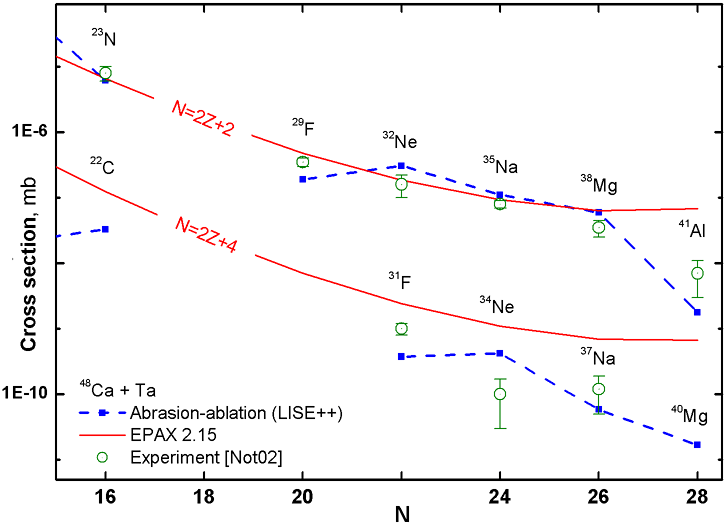
Table 12. Parameters of Abrasion-Ablation model were used in calculations in Fig.34.
Fig.34. Experimental [Not02,Sak97], calculated by the LISE abrasion-ablation model (blue dash curve) and EPAX parameterization (red solid curve) production cross sections of neutron-rich isotopes in the reaction 48Ca+Ta versus neutron number. Binding energies from the database+LDM2 have been used for abrasion-ablation calculations. More detailed description of improved mass
parameterizations will be given in the upcoming paper [Sou02]. 6. Updating and new utilities
6.2. PreferencesIn LISE++ the
dialog “Preferences” has got a number of new options some of them already
were described above. There are just some words about the new option “Calculate
spectrometer setting using maximal or mean value of the momentum
distribution”. The rigidity can be calculated using one of conditions (see Fig.36): ·
The maximum of momentum
distribution corresponds to the central line of the spectrometer (left plot),
·
The average of momentum
distribution is in the central line (right plot). This is the new feature of
the code. The program LISE assumed only the first case for calculations.
6.4. Dialogs Goodies & Physical calculatorIn the dialog “Goodies” the code calculates standard deviations of times of flight and energy loss in materials. Momentum acceptance and detector (timing, energy) resolutions are taken into account.
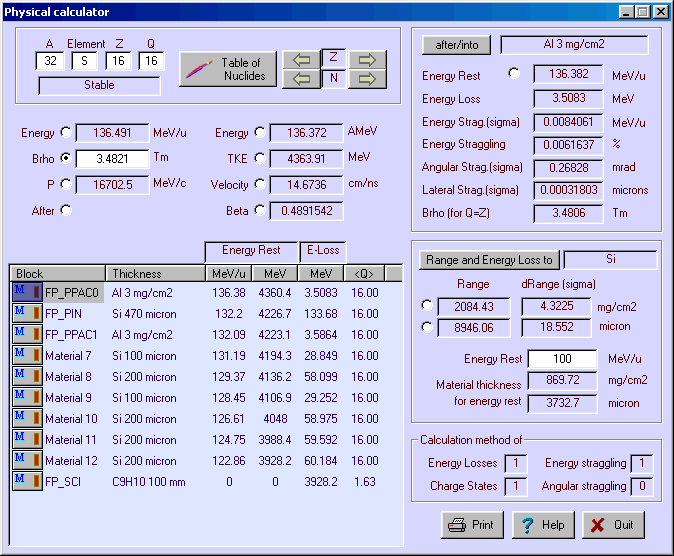
Fig.38. Physical calculator. The Physical calculator of LISE++ can calculate energy loss throughout unlimited number of detectors (see Fig.38). The number of detectors in LISE was limited to seven. It is possible to edit materials without leaving the physical calculator dialog by clicking on an icon of a detector in the window of materials. G The window of material blocks contains only
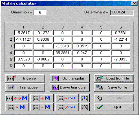
materials located after the last optical block. Lateral straggling through materials is included in the physical calculator, which is calculated on the basis of angular straggling and the detector length. The lateral straggling of fragments through a material is taken into account in fragment transmission calculations. The biggest effect of lateral straggling can been seen in for gas detectors. 6.5. Matrix calculator
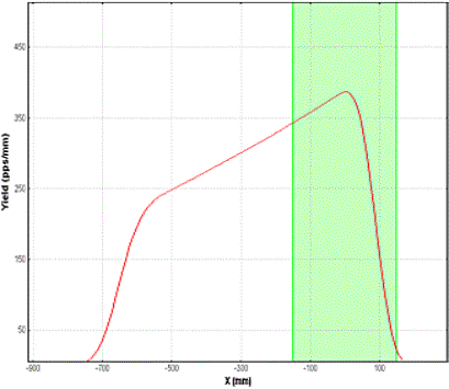
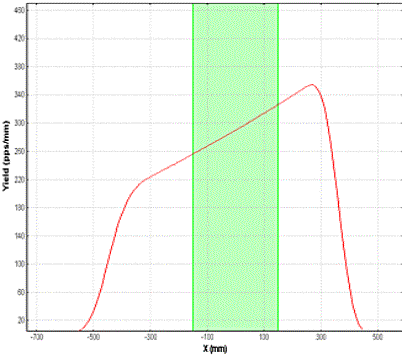
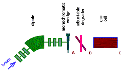
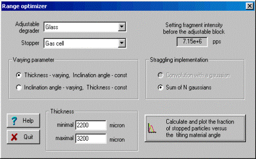
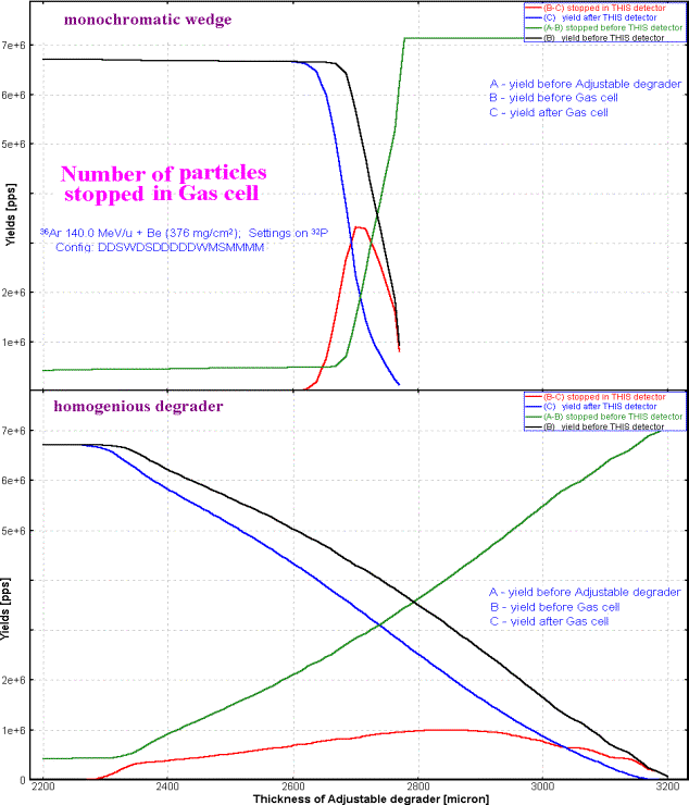
The user has to choose, in the range optimizer dialog, the adjustable degrader material, the stopper material and the minimum and maximum thicknesses of the adjustable degrader. The code automatically suggests the minimum and maximum thicknesses of the adjustable degrader equal to zero and the range of the particle in the adjustable degrader respectively. The number of points used to calculate the optimal thickness (inclination angle) is equal to the number of points for the optimal thickness target calculation utility defined in the Preferences dialog. The number of particles stopped in the gas cell versus the thickness of the adjustable degrader for two different wedges before the adjustable degrader are shown in Fig.42. It is visible from the figure that it is possible to set the adjustable degrader, using the monochromatic wedge, to stop 3.5 times more particles in the gas cell if a homogeneous degrader is used.
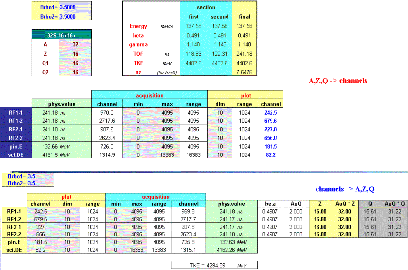
Fig.42. Number of particles stopped in the gas cell versus the thickness of adjustable degrader for two different wedges before the adjustable degrader (see the scheme in Fig.40). The case of the monochromatic wedge is shown in top plot, the homogeneous degrader is given in the bottom plot. 6.7. LISE for ExcelThe new version of LISE.xls allows you to make a fast identification of isotopes and a calibration of experimental registered parameters during an experiment. For calibration and identification LISE.xls uses the configuration: Dipole Þ Wedge Þ Dipole Þ dE-detector Þ TKE-detector Initially, it is necessary to input parameters of a set-up (lengths of dispersive blocks, dE-detector properties, etc) and perform calibrations of time-of-flight and energy loss in the dE and TKE detectors. You can use the new utility in two directions: · Input parameters A, Z, Q1 and Q2 of the isotope of interest and input the Brho values to get energy loss and time-of-flight data in channels (upper picture in Fig.43); · Input experimental data in channels to get physical values (energy loss and time-of-flight) and identification of the ion (lower picture in Fig.43). You can only edit cells with a light grey background (see Fig.43). Other cells are write protected.
Fig.43. New
identification tables of LISE.xls. New transformation functions (Energy Û Momentum, Brho Û Momentum) and some new statistic functions (integration, etc) have been incorporated in the LISE.xls package. One improvement is that LISE.xls can handle unphysical inputs (i.e. a negative value for a material thickness).
7. PlotsThe program can plot angular, spatial, energy and momentum distributions before and after every block, as well as inside a dispersive block. It permits to the user to look at how the dynamics of distributions change from block to block. Two-dimensional plots allow the user to see correlations between parameters (dE, TKE, TOF, X, Y) in detectors with the resolution of detectors taking into account. 7.1. Transmission plots
One-dimensional selection
plots can be found through the menu “Plots” or the LISE++ toolbar. Table
13 shows different types of selection plots. Momentum
and Vertical special selection plots are available only from the menu “Plots”. By clicking the icon of any of
the plots (except for the Brho and Wedge selection plots) in the toolbar you get
the menu of available blocks for which can be constructed the plot. The Brho
and Wedge selection plots are drawn immediately, without this menu, for
blocks, which were set in the dialog “Plot options” (Fig.45). If the plot selection window has more than one
plot then you can use the button Table 13. Selection plots.
Fig.45. The
“Plot options” dialog. 7.2. Two-dimensional plotsThe use of experimental data from different detectors to build a two-dimensional plot is a large advantage of LISE++. For example, you can build a two-dimensional plot using the Х-coordinate from a PPAC located in Image2 and an energy loss value from a PIN-detector located after the last optical block. First you have to set in the "Plot options" dialog (Fig.45) “PPAC in Image2” as the X-detector and “PIN-detector” as the dE-detector. Then you click on plot "dE-X" from the menu "Plots" to create the plot. Material (detector) blocks only can be used to make two-dimensional plots. The code
uses a trigger for data acquisition taken from a detector. For
"ellipse" mode drawing of two-dimensional plots, the first detector
found in the beam line is used. For Monte Carlo simulations the last detector
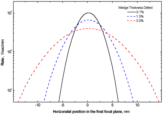
is used to start an acquisition. Energy, time, and spatial resolutions of a detector are used when calculating standard deviations of measured values in two-dimensional plots. The defect (percent error) of a material thickness is used in two-dimensional plots as well as in fragment transmission calculations. You can see the increase in a peak width with a larger detector resolution or larger material thickness defect.
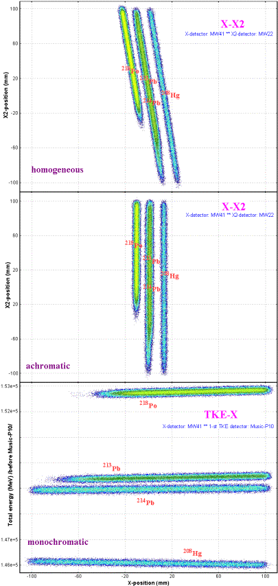
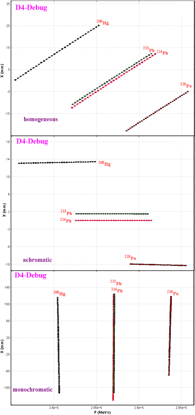
7.3. Debug distributionsDebug distributions serve to check transmission calculations and transformations of distributions and represents an ideal transformation of the momentum to a coordinate. The given distribution (PÞx) is used in convolutions with spatial (x) and angular (qÞx) components to get an output spatial distribution after a block. Using debug distributions it is easy to see the dependence of distributions on wedge shape. Debug distributions also can be used for calculation of achromatic or monochromatic wedges (see the lower right plot in Fig.21). Fig.47 shows two-dimensional spectra for the reaction 238U(1 GeV/u) + Be(3.5 g/cm2)Þ 214Pb
with a Al 1 g/cm2 wedge found between the 2nd and 3rd dipoles
of the fragment separator FRS. The spectra are calculated for different wedge
shapes. Fig.48 shows debug distributions after the 4th
dipole for the same reaction as in Fig.47. Only calculations for isotopes 208Hg, 213,214Pb, 218Po
are shown in the plots for illustration purposes. This example is available
through the LISE web-site: http://lise.nscl.msu.edu/6_1/examples/214pb.lpp The debug information window (the menu “PlotÞDebug information”) as well as debug distribution plots are only used for the developers of the program to control calculations of standard deviations of the main characteristics of debug distributions.
8. Future developments of LISE++· Develop new dispersive blocks: gas-filled, electrostatic separators, compensating dipole after the Wien velocity filter. · Create LISE++ configuration files for spectrometers in GANIL, Dubna, RIKEN, Texas A&M, etc. The authors hope to have help from experts of these laboratories for specific information (transport files, location and characteristics of detectors, emittance of primary beam, etc.). · Add a subroutine of fusion cross-section calculations below the Coulomb barrier in the PACE4 code and the LisFus model of LISE++. · Incorporate a new reaction mechanism: Fission (principal task for 2003 FY) · Develop a new material block: secondary target · Continue work under “Universal parameterization of momentum distribution of projectile fragmentation products”. · Write a guide, “First steps” for beginners. · Write full LISE++ documentation. · Develop the “Beam analyzer” dialog to plot beam trajectories in dipoles. Acknowledgements
LISE++ authors gratefully acknowledge Dr.Helmut Weik’s fruitful remarks, suggestions, and help with the development of LISE++. Special thanks to Helmut for continually checking the code. LISE++ authors thank Heather Olliver for carefully proof reading this manual. Fruitful discussions with Prof.Betty Tsang on the improved masss formula (chapter 5.) and with Dr.Leo Weissman on the gas cell range optimizer (chapter 6.5.) are gratefully acknowledged. The authors are grateful to the entire National Superconducting Cyclotron Laboratory for fuitfull remarks, comments and checking of preliminary versions of LISE++. References:
[Aud95] G.Audi and A.H.Wapstra, Atom.Data and Nucl.Data Tables (1995) 1. [Bro80] K.L.Brown et al. CERN 80-04 (1980); [Kra87] ”Introductory nuclear physics”, K.S.Kraine,
publ. By John Wiles & sons, New York, 1987. [Mye66] W.D.Myers and W.J.Swiatecki, Nuclear Physics
81(1966) 1-60. [Not02] M.Notani et al.,
Phys.Lett.B, in press. [Sak97] H.Sakurai et al.,
Nucl.Phys. A616 (1997) 311c. [Sou02] “Improved mass
parameterization in reaction models”, S.R.Souza et all. To be published. |
|||||||||||||||||||||||||||||||||||||||||||||||||||||||||||||||||||||||||||||||||||||||||||||||||||||||||||||||||||||||||||||||||||||||||||||||||||||||||||||||||||||||||||||||||||||||||||||||||||||||||||||||||||||||||||||||||||||||||||||||||||||||||||||||||||||||||||||||||||||||||||||||||||||||||||||||||||||||||||||||||||||||||||||||||||||||||||||||||||||||||||||||||||||||||||||||||||||||||||||||||||||||||||||||||||||||||||||||||||||||||||||||||||||||||||||||||||||||||||||||||||||||||||||||||||||||||||||||||||||||||||||||||||||||||||||||||||||||||||||||||||||||||||||||||||||||||||||||||||||||||||||||||||||||


 [J/C]
[J/C]