|
The code LISE: version 4.18 |
|
lise.nscl.msu.edu
|
East Lansing
|
Evaporation Calculator
Abrasion-Ablation Model
Contents:
1. Introduction
2. Evaporation Calculator
2.1. Evaporation calculator plots
2.2. Evaporation settings
2.2.1. Tunneling for charge particles
2.2.2. Option to take into account unbound nuclei
3. Geometrical Abrasion-Ablation Model
3.1. Abrasion-Ablation settings
3.1.1. LISE corrections
3.1.2. Excitation energy
Epilogue
References
Various versions of the EPAX parameterization [Sum00] have been used to calculate projectile fragmentation cross-sections. The basic advantages of the parameterization are the following:
However, there are some disadvantages:
In further developments of the program LISE other kinds of reaction, in addition to projectile fragmentation will be introduced. One candidate is complete fusion with subsequent evaporation and/or fission. These reactions require an in built procedure for calculating light particle evaporation by exited nuclei.
This has resulted the creation of a new calculator called "Evaporation Calculator" [Chapter 2.]. Using this new tool the user can calculate the production cross-sections of different nuclei as a result of deexcitation of an excited nucleus. This calculator is based on the work by [Gai91]. The introduction of the evaporation algorithm allows incorporation of an additional method for calculating projectile fragmentation cross section using an Abrasion-Ablation model [Chapter 3.].
2. Evaporation Calculator
The Evaporation calculator is available in the Calculations menu or via the icon ![]() in the toolbar (see Fig.1). The "Evaporation Calculator" dialog is shown in Fig.2. The production of 32Mg nucleus from deexcitation of 40Ar is presented in this figure as an example. The excitation energy
distribution of 40Ar in this example is gaussian, with the excitation energy window (50 MeV, 100 MeV)
as the left and right points at the gaussian half-height.
in the toolbar (see Fig.1). The "Evaporation Calculator" dialog is shown in Fig.2. The production of 32Mg nucleus from deexcitation of 40Ar is presented in this figure as an example. The excitation energy
distribution of 40Ar in this example is gaussian, with the excitation energy window (50 MeV, 100 MeV)
as the left and right points at the gaussian half-height.
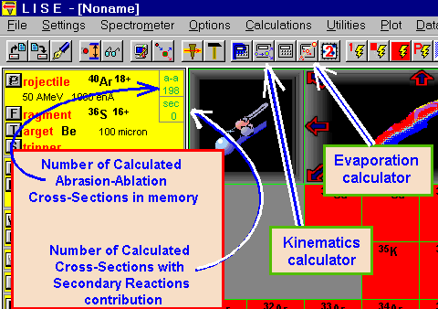
Fig.1. Icons of Kinematics and Evaporation calculators.
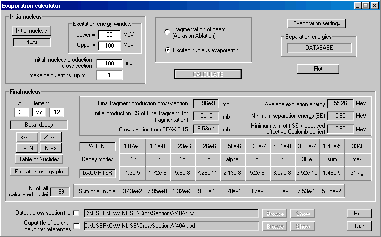
Fig.2. The "Evaporation Calculator" dialog (Excited 40Ar nucleus evaporation example).
The basic differences between the work [Gai91] and the LISE algorithm are the following:
In this sense the LISE method is unique: it carries in itself the best features of Monte Carlo evaporation programs (energy distributions, odd-even effects, "individuality" of each nucleus) and one of the advantages of analytical methods [Gai91] - fast calculations.
2.1 Evaporation calculator plots
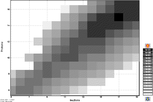
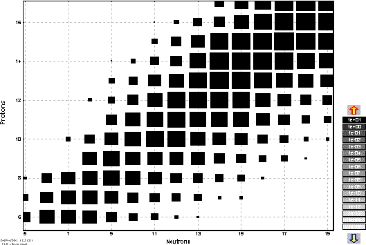
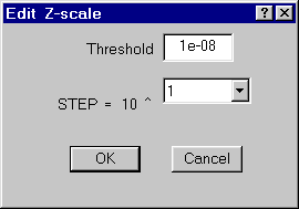
The user can observe results of the evaporation calculator using plots of input and output energy distributions for a given nucleus (see Fig.3) and a two-dimensional plot of cross-sections (see Fig.4). The 2D-dimensional plot is a new feature in the program. The data is represented by rectangles centered at N (neutrons) and Z (protons), where the cross-section value depends on color and size of the rectangle. The user can change the display modes of rectangles (see Fig.5), and also change the scale (see Fig.6).
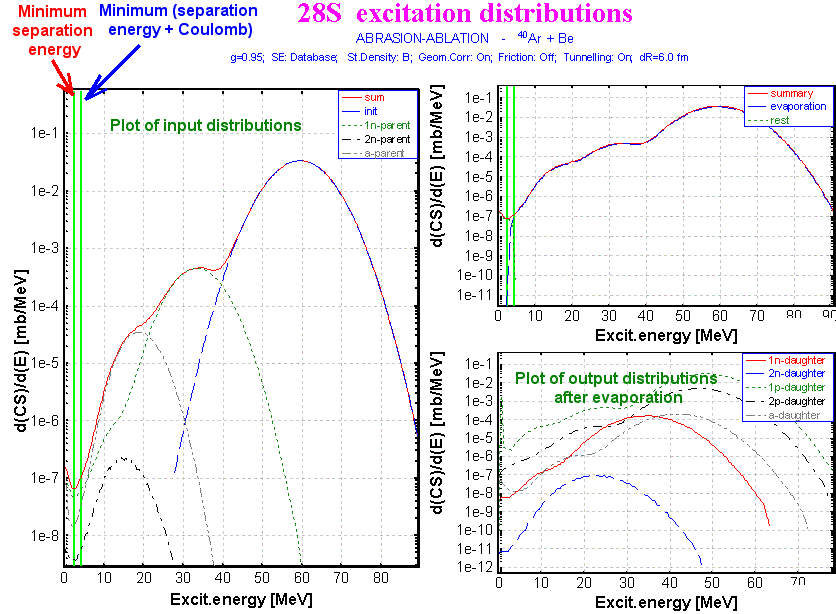
Fig.3. Parent (input) and Daughter(output) distributions of 28S nucleus in the reaction 40Ar+Be. These plots are available via the "Excitation energy plots" button in the "Evaporation calculator" dialog.
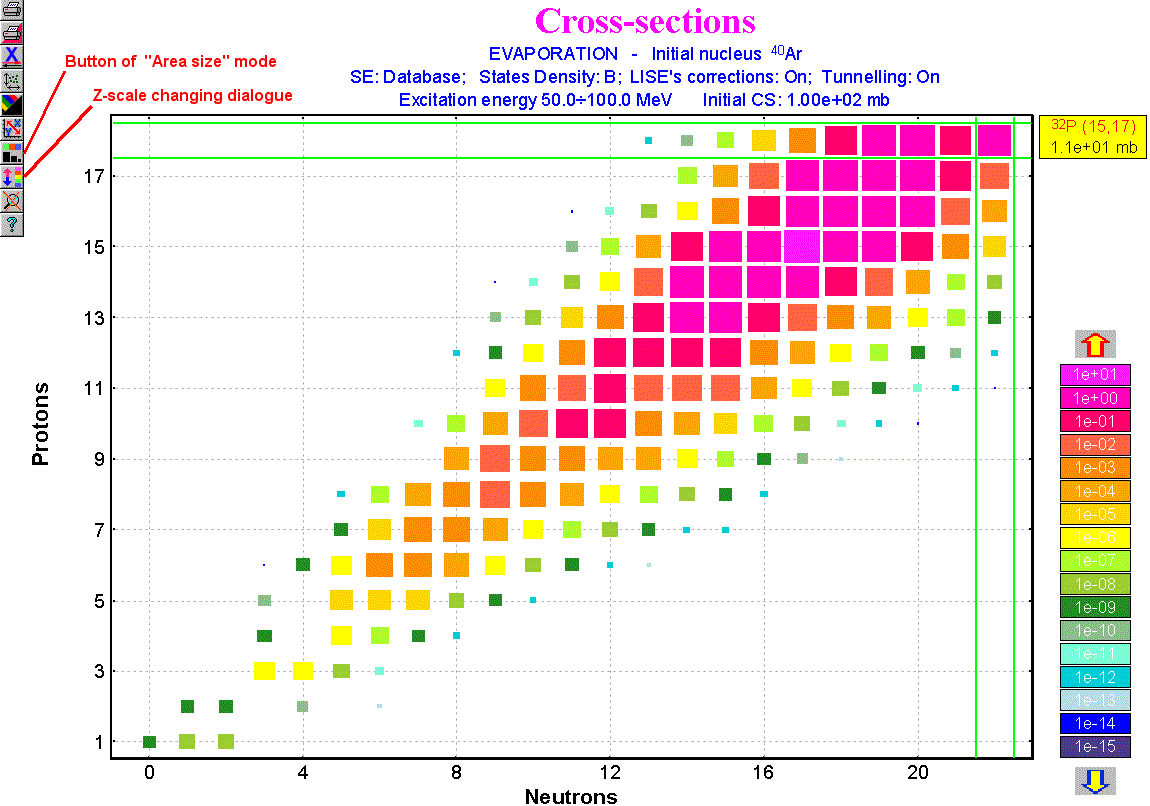
Fig.4. The bi-dimensional plot of production cross-sections of nuclei as a result of 40Ar deexcitation.
|
|
|
|
Fig.5. Different presentation modes of the new bi-dimensional plot. |
|
2.2 Evaporation settings
| The "Evaporation settings" dialog (see Fig.7) can be accessed from the "Evaporation calculator" dialog or from the "Options" menu. Eight decay modes are available in the code. The user can not
change three of them (p,n,a
). Other modes may be switched on or off. It is not recommended to use 3He and t —decays as their contributions are insignificant, and increases calculation speed. The user can test this by perfoming calculations with various options. |
Fig.6. The dialog “Edit Z-scale”. |
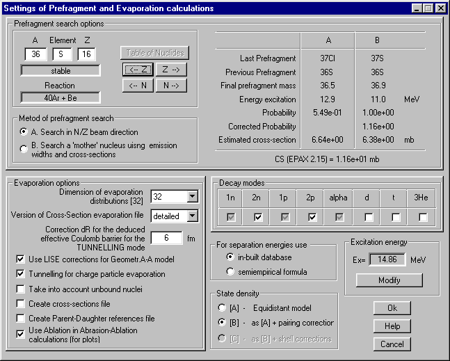
Fig.7. Settings of Prefragment and Evaporation calculations. (Recommended values are shown)
2.2.1 Tunneling for charge particles
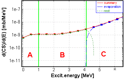
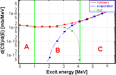
In Fig.3 and Fig.8 plots are shown with two green vertical lines corresponding to the minimum separation energy (left line) and the minimum sum of the separation energy and the effective Coulomb barrier (right line). The part of the distribution (A) located to the left of a line does not undergo evaporation (see Fig.8). The deexcitation proceeds by emission of g -rays. It is also assumed, that the part of the distribution between these two lines (B) does not undergo the further evaporation (see Fig.8, left plot). The effective barrier assumes a shift of the right line to the left, assuming a tunneling effect. The default value dR = 6 fm is taken from work [Ben98]. The effective Coulomb barrier is written as:
![]() . /1/
. /1/
|
|
|
|
Fig.8. Excitation energy distribution plots. The left plot shows the calculation principle in the LISE code. The right plot is an idealized case, which is still in a stage of development. |
|
In Fig.8 (right plot) an example of a real situation including a tunneling effect is shown (this is still in a stage of development). Not all part would remain in the given fragment in this case in the B zone. The standard Coulomb barrier is used in this case:
![]() .
/2/
.
/2/
The use of the effective barrier can have various consequences. For example, when the sum of the separation energy and the Coulomb barrier is positive, the nucleus is bound. However it is not excluded that at the same time the sum of the separation energy and the effective Coulomb barrier is negative (as the effective Coulomb barrier is less the standard barrier). In this case the nucleus is unbound and the program will show zero cross-section for its production.
2.2.2 Option to take into account unbound nuclei
This option includes calculating unbound nuclei suggesting via evaporations channels, for example, the most probable path of 32Ne nucleus deexcitation is 32Ne*-> 31Ne-> 30Ne in the 40Ar+Be reaction. This option brings contribution for nuclei near the drip-lines. Cross-sections of 24O, 29F, 30Ne are increased about 1-3% with this option from a test in the 40Ar+Be reaction.
3. Geometrical Abrasion-Ablation Model
In the LISE code, a simple theory of fragmentation based upon a two-step abrasion/ablation model is presented [Wil87]. The abrasion process accounts for removal of nuclear matter in the overlap region of the colliding ions. An average transmission factor is used for the projectile and target nuclei at a given impact parameter to account for the finite meanfree path in nuclear matter. The ions are treated otherwise on a geometrical basis assuming uniform spheres. The surface distortion excitation energy of the projectile prefragment following abrasion of nucleons is calculated from the clean-cut abrasion formalism of [Gos77]. Wilson’s model also includes (see Chapter 3.1.2. Excitation energy):
3.1 Abrasion-Ablation settings
User may access the abrasion-ablation setting via the "Evaporation settings" dialog (see Fig.7).
3.1.1 LISE corrections
There are restrictions in the geometrical abrasion-ablation model when light targets are used. For example, it is impossible to get a prefragment mass less than 22 in the 40Ar+Be reaction. In other words the target cannot in this geometrical assumption make an aperture in a particle more than the volume proportional to mass 18 nucleons. Further prefragment deexcitation will not allow to be lowered more than on 5 units, though in experiments all spectrum of elements inclusive up to hydrogen is observed (see Fig.9). Corrections have been incorporated in the program LISE to solve this restriction. The code extrapolates exponentially the dependences of cross-sections and excitation energies from the prefragment mass in the break point in a lightest targets case (Fig.10).
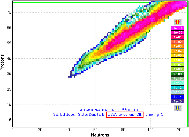
Fig.9. Cross-sections plot for the 208Pb + Be reaction. LISE corrections for Geometrical Abrasion-Ablation model are switched OFF.
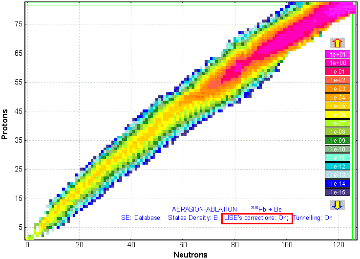
Fig.10. Cross-sections plot for the 208Pb + Be reaction. LISE corrections for Geometrical Abrasion-Ablation model are switched ON.
3.1.2 Excitation energy
The user can vary excitation energy options in the "Excitation energy of prefragment" dialog (Fig.11). This dialog is available the "Options" menu or the "Evaporation settings" dialog (see Fig.7). The excitation energy calculation is based on the work of [Wil87].
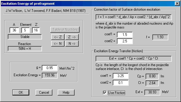
Fig.11. Prefragment excitation energy settings.
The user can change coefficients of correction factors in this dialog. Original coefficients in the work [Wil87] for correction factor expression (17) are 15 and 25. We assume, that these coefficients are erroneous. Real values should be in the range 1.5 and 2.5 correspondingly. For example, if to suggest a projectile half-part abrasion the correction factor will be equal to 14.75! Comparing excitation energy with the work [Gai91], more real vale of the correction factor should be about 2.
Two additional methods of excitation energy calculation are planed in the next version. The first method is based on the diabatic model [Gai91] (convolutions of several linear distributions), the second one is a simplified approach from the first method:
![]() .
/3/
.
/3/
Cross-sections calculated by the abrasion-ablation model may be used for other calculations into the program (see Fig.12). Cross-sections are saved in the memory (see Fig.1) and will be recalculated if the projectile (target) is changed.
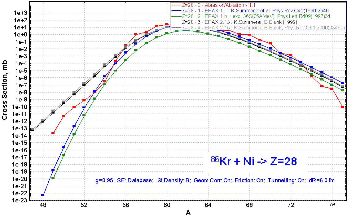
Fig.12. Prefragment excitation energy settings
All remarks, comments for the Evaporation calculator and Abrasion-Ablation model are welcome!
[Ben98] J.Benlliure et al., Eur.Phys.J. A 2 (1998) 193.
[Gai91] J.-J.Gaimard, K.-H.Schmidt, Nucl.Phys. A531 (1991) 709-745.
[Gos77] J.Gosset et al., Phys.Rev. C16 (1977) 629.
[Sum90] K.Sümmerer et al., Phys.Rev. C42(1990)2546-2561.
[Wil87] J.W.Wilson, L.W.Towsend, F.F.Badavi, NIM B18 (1987) 225-231.