Table of Contents
LISE++ Ray Reader Documentation
Brief Overview
The LISE++ Ray Reader is a plotting tool that takes Monte Carlo simulated data from the LISE++ program and plots it using Matplotlib in python. Allows for 1-D, 2-D, and 3-D plots to be compared simultaneously. Matplotlib plots can be saved and stored on a local computer. The LISE++ Ray Reader program can be downloaded from the LISE++ nscl.msu.edu website.
LISE++ Ray Reader is a stand alone utility that analyzes a comma delimited .ray file that is generated through the Monte Carlo fragment transmission simulator within LISE++. The Ray Reader program creates 1D, 2D, and 3D plot graphics that can be used for Power Point presentations, web graphics, reports, and other academic uses. The data within the .ray file can be manipulated by selecting specific locations and fields in combo boxes that can be filtered by restricting the data numeric values. The Ray Reader can generate five different plots simultaneously, the 1D (X, Y, and Z), 2D (X/Y), and 3D (X/Y/Z). The data results will also display in a "Data results" tab. Each of the five plots can have unique styles set such as the plot color, marker, and edge. At the time this documentation was written, the version of LISE++ was 16.3.7. This documentation is written for the Ray Reader version beta 1.0.
All data examples used in this documentation are specific to the A1900 fragment separator.
Ray file creation
In order for this program to function properly, create a ray file from the LISE++ program.
Step by step instructions from LISE++
Step 1: Launch LISE++. If you don't have it download it here.
Step 2: Click the preferences icon ![]() that is fourth from the left at of the top tool bar.
that is fourth from the left at of the top tool bar.
 Top
Top
Step 3: Select the configuration file and options file you want. In our case we selected the A1900 fragment separator which is the default option.
 Top
Top
Step 4: Select experimental parameters located in the yellow section.
 Top
Top
Step 5: Select the "all nuclei" button ![]() that is twelfth from the right in the top tool bar once experimental parameters are selected. The table of nucleides will be empty before pressing the "all nuclei" button.
that is twelfth from the right in the top tool bar once experimental parameters are selected. The table of nucleides will be empty before pressing the "all nuclei" button.
 Top
Top
Step 6: Select the Monte Carlo icon ![]() that is second from the right in the top tool bar.
that is second from the right in the top tool bar.
 Top
Top
Step 7: Select the radio button for the "Group of isotopes already calculated by the Distribution method."
 Top
Top
Step 8: Click the "MC transmission options" towards the bottom-left of the "Monte Carlo calculation of fragment transmission" box.
 Top
Top
Step 9: In the "MC transmission options" box to the top-right check the box next to "Cross-sections independent calculations (all cross section equal)."
 Top
Top
Step 10: Select the "MC calculation to file" at the bottom-left corner of the "Monte Carlo calculation of fragment transmission" box.
 Top
Top
Step 11: Select locations to perform Monte Carlo simulation. In the locations combo box you can enter the number of locations you want. The example shown is for the A1900 fragment separator.
 Top
Top
Step 12: Select fields to perform Monte Carlo simulation. In the fields combo box you can enter the number of fields you want. The example shown is for the A1900 fragment separator.
 Top
Top
Step 13: To the bottom right of the "Rays generator" window select the comma option under the "Fields separator" drop down box.
 Top
Top
Step 14: Click the Run button at the bottom left of the "Rays generator" box. You will see the file being generated indicated by the box saying "Generating Ray file." The "Isotope Group: Monte Carlo Transmission Plot" can be ignored. The save path on windows will be C:\Users\<user>\Documents\LISEcute\files.
 Top
Top
Optional Step: If the user wished to rename the file or change where the ray file is saved you can click the "Output file name" button. The "Save As" box will show the directory where the ray file will be saved and the name of the file can be changed. It will automatically save to C:\Users\<user>\Documents\LISEcute\files with the file name "MC_LISE.ray." The first graphic below shows where to select the output file. The second graphic below shows the "Save File" dialogue box that appears when the "Output file name" button is clicked.

 Top
Top
Plot settings
The plot settings contain all the parameters necessary for plotting the simulated output produced from the LISE++ program. The main data is measured at the Locations and Fields that is simulated from the actual facility of interest.
Locations
The locations refer to individual portions of the fragment separator of interest. The following graphic is a snapshot of the A1900 fragment separator displayed in the LISE++ program.
 Top
Top
The list below defines each point in the A1900 fragment separator.
- Target: The physical target that the beam fed from NSCL hits to produce isotopes.
- D1, D2, D3, and D4: Dipole magnets that direct the beam line.
- I1, I2, and FP_Slits: Adjustable slits on the fragment separator.
- FP_PPAC0 and FP_PPAC1: Two-dimensional position sensitive parallel-plate avalanche (PPAC) detectors.
- FPIN: The detector using a PIN diode (p-type, intrinsic, n-type diode) at the focal plane.
- FP_SCI: The final location of the fragment separator.
The user can select a location from the combo boxes in the "Locations" section. These locations are pulled from the .ray file that is generated from LISE++. The graphic below shows the X values in the combo box that was loaded from the ray file "ray-tutorial.ray."
The location values will be the same in every location combo box throughout the program. The location values come from the .ray file that was generated within the Monte Carlo simulation in the LISE++ program.
 Top
Top
Fields
The fields in the combo box are taken from the .ray file that is generated from the LISE++ Monte Carlo simulation of the fragment transmission. These parameters will load into the Ray Reader Fields combo box. An example list of available values for the A1900 fragment separator are defined below.
- X [mm]: The physical horizontal distance of the particle from the location in millimeters
- X'(Theta) [mrad]: Polar angular distance from location
- Y [mm]: The physical vertical distance of the particle from the location in millimeters
- Y'(Phi) [mrad]: Azimuthal angular distance from location
- dP/P [%]: Ratio of the change of momentum to the total momentum of the particle
- Radial [mm]: The radial distance from location in millimeters
- Angle [mrad]: The angle in milliradians
- Energy [MeV/u]: The mega electron volts of energy per unified atomic mass unit of the particle at the specified location
- TKE [MeV]: Total Kinetic Energy of the particle at the location
- Momentum [GeV/c]: The physical momentum of the particle at the location
- Brho [T*m]: The magnetic rigidity of the location
- Erho [MJ/C]: The electrostatic rigidity of the location
- Length from Target [m]: The physical distance from the target to the location in meters
- Time from Target [ns]: The time the particle takes from target to location in nanoseconds
- Energy Loss (MeV): How much mega electron volts of energy is lost from the time from the target to the location in the detector.
- Range (mm): The range of the particle at the location in millimeters
- Reaction: Measures the reaction mechanism of the nucleides
- Cross Section (mb): The probability of two particles at the target producing a reaction millibarns
- Velocity [cm/ns]: Speed of the particle at the location in centimeters per nanosecond
- Velocity_Z [cm/ns]: Speed of the particle at the location in centimeters per nanosecond in the Z direction
- Velocity_X [cm/ns]: Speed of the particle at the location in centimeters per nanosecond in the X direction
- Velocity_Y [cm/ns]: Speed of the particle at the location in centimeters per nanosecond in the Y direction
- Velocity_XY [cm/ns]: Speed of the particle at the location in centimeters per nanosecond in the X and Y direction
- Beta: The relativistic speed of the particle at the location
- Gamma: The Lorentz factor of the particle at the location
- Mass (amu): The atomic mass units of the particle at the location
- A (mass number): Atomic mass number of the particle at the location
- Z (atomic number): Atomic number of the particle at the location
- N (neutron number): Neutron Number of the particle at the location
- q (ion charge): The ion charge of the particle at the location
The field values will be the same in every field combo box throughout the program. The field values come from the .ray file that was generated within the Monte Carlo simulation in the LISE++ program.
TopThe graphic below shows what the fields look like after the .ray file is loaded.
 Top
Top
Data range filter
The "Data Range Filter" filters the data results to specific parameters. The data results can be narrowed down to a specific location, field, and numeric value range.
DRF Locations
The "Location" combo box are the same as found in the Locations section. The "Locations" combo box is to allow the data set to be filtered to a specific range of data. This narrows the data results to a specific location within the fragment separator that is not necessarily the X, Y, or Z location chosen in the data sample you are plotting. For example in the graphic below , the X, Y, and Z locations are set to the location within the A1900 FP_PIN detector. The location selected in the "Data Range Filter" is selected to the location where the I1_Slits are within the A1900 fragment separator.
 Top
Top
DRF Fields
The "Fields" combo box are the same as found in the Field section. Similar to the "Locations" in the previous section, the "Fields" can be filtered to a specific field quantity that is measured at the specific location. The graphic below shows where the "Data Range Filter" Field combo box is located.
 Top
Top
DRF Boundary Slider
The boundary slider can filter the data results by the lowest negative and greatest positive number. You adjust the numeric value by dragging the slider handle or by clicking in the grayed out area of the slider. Moving the handle increments at a greater rate that clicking the gray area of the slider. Clicking the gray area will increment by 1 value per click. The below graphic shows the location of the boundary slider.
 Top
Top
Plot Style Settings
The "Plot Style Settings" allow the user to customize the appearance of each graphic individually on each tab.
Color map
The color map combo box contains a various array of color styles that are supplied by the matplotlib documentation. The graphic below shows the available colormaps in the Ray Reader program combo box.
 Top
Top
Only a few of the possible colormaps available are supplied in the Ray Reader program. The below graphics are the key to the colormaps that are available in the Ray Reader program.
For a full list of color map style please visit the matplotlib colormap reference.


Marker
The markers used in the LISE++ Ray Reader is from Matplotlib's library. The table below is from the Matplotlib Documentation. For a comprehensive list of the marker styles, please visit the Matplotlib website regarding matplotlib.markers.
marker |
symbol |
description |
|---|---|---|
|
|
point |
|
|
pixel |
|
|
circle |
|
|
triangle_down |
|
|
triangle_up |
|
|
triangle_left |
|
|
triangle_right |
|
|
tri_down |
|
|
tri_up |
|
|
tri_left |
|
|
tri_right |
|
|
octagon |
|
|
square |
|
|
pentagon |
|
|
plus (filled) |
|
|
star |
|
|
hexagon1 |
|
|
hexagon2 |
|
|
plus |
|
|
x |
|
|
x (filled) |
|
|
diamond |
|
|
thin_diamond |
|
|
vline |
|
|
hline |


Style Location
The "Location" combo box in the "Data Range Filter" allows the user to apply a colormap to your plots based on a different location that is specified in the X, Y, and Z Value columns. The graphic below shows where the "Location" combo box is in the "Data Range Filter."
 Top
Top
Style Field
The "Field" combo box in the "Data Range Filter" allows the user to apply a colormap to your plots based on a different field that is specified in the X, Y, and Z Value columns. The graphic below shows where the "Field" combo box is in the "Data Range Filter."
 Top
Top
Edge
The "Edge" combo box shown in the graphic below adds an outline to each individual plot marker.

The below graphic shows what the edge looks like when a "black" edge is applied to the "gist_rainbow" colormap.
 Top
Top
Plot Style Examples
The following graphics show examples of each tab in order of how the colormap, marker, location, field, and edge parameters are displayed when plotted. Each tab can be customized particularly to its own requirement and displayed simultaneously.


 Top
Top
Plot Analysis Window
The "Plot Analysis Window" displays the data results and the 1D, 2D, and 3D plots in separate tabs.
"Data results" tab
The "Data Results" tab contains the data that was plotted from the .ray file.
 Top
Top
When the data is filtered using the "Data Range Filter" only the filtered data will appear in the "Data Results" tab. Below is a graphic of filtered data in the "Data Results" tab.
 Top
Top
"X plot", "Y plot", and "Z plot" tabs (1D)
The X, Y, and Z plots function the same. The "X Value" column in the "Plot Settings" will display in the "X Plot" tab, the "Y Value" column will display on the "Y Plot" tab, and the "Z Value" column will display in the "Z Plot" tab. These are the same data columns shown in the "Data Results" tab. The below image is the default style the user will see with no style changes.
 Top
Top
"X and Y plot" tab (2D)
The X and Y columns in the "Plot Settings" will be combined in the "X and Y plot" tab. The following graphic is a default styled 2D X and Y plot.
 Top
Top
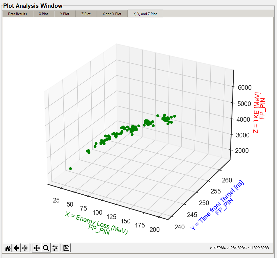
"X, Y, and Z plot" tab (3D)
The 3D plots are a combination of the X, Y, and Z Values in the "Plot Settings." The below graphic is a default 3D plot with no style applied.
 Top
Top
How to use Matplotlib plot window
The Matplotlib controls are located at the bottom left hand side of the plot window.
Reset
When changing the views of your particular plot, you can reset the view to the default position by clicking the "Reset" button shown in the graphic below.

Top
Previous and Forward
The previous and forward buttons will allow the user access a history of views that were created in order. When the arrows are blanked out like the following image, there were no views made.
When you have zoomed, panned, or made a change in the view, the left arrow will become dark.
If you made multiple changes, both arrows will become dark indicating that you can go forward or backward in the order of the history of changes.
Top
Pan
The plot can be panned in various directions, the "Pan" button is shown in the following graphic.

1D and 2D pan left and right
The default position prior to panning left or right is shown below.

You can pan left, right, up, or down.
First, click the "Pan" button.
Then hold the left mouse button down and move the cursor in the direction you wish to pan towards.
The first graphic on the bottom shows a pan to the left and the second bottom graphic shows a pan to the right.

 Top
Top
3D pan
You can also pan the 3D graphic in any direction 360 degrees using the same method as the 1D and 2D pan.
First, click the "Pan" button.
Then hold the left mouse button down and move the cursor in any direction you wish to pan towards.
The first graphic below shows an upwards pan and the second graphic shows a left pan.

 Top
Top
Zoom
You can zoom into your plot by using the "zoom" tool button shown in the graphic below.

1D and 2D plot zoom
After selecting the zoom button, you can use the square marquee to select the area you want to zoom into. The first graphic below shows the marquee tool in use. The second graphic below shows the plot after the area was selected by the zoom tool.

 Top
Top
3D plot zoom
To zoom into a 3D plot, hold the right mouse button down and move your mouse up (zoom in) or down (zoom out). The first graphic below is zoomed in and the second graphic is zoomed out.
If your mouse has a scroll wheel, you can use the scroll wheel to zoom in and out as well.

 Top
Top
Configure Subplots
You can adjust the view of each subplot configuration using the "Configure Subplots" button. The "Configure Subplots" button is displayed in the following graphic.

Clicking the "Configure Subplots" button brings up the "Subplot Configuration Tool" shown in the graphic below.

You can adjust the left, bottom, right, top, wspace, and hspace by moving the slider handles left or right.
TopSave
You can save your plot graphic by clicking the "Save" button shown in the graphic below.

When you click the "Save" button, a "Save the figure" dialogue box will appear allowing the user to choose the location, file name, and file type. You can save each plot as a .png, .jpg, .jpeg, .eps, .pdf, .pgf, .ps, .raw, .rgba, .svg, .svgz, .tif, or .tiff file format.
TopTroubleshooting
The Ray Reader program has a console running in the background that provides meta data while the program runs. The user can use this to diagnose errors while using the program.
TopConsole
The Ray Reader program also has a console running in the background in order to view raw data statistics and errors. When the program initially loads, there will be no .ray file data loaded. The below graphic shows the console at the initial state.

When a .ray file is loaded, the console will display the data from the .ray file. The below graphic shows what the .ray file data looks like in the console.
 Top
Top
FileNotFoundError: [Errno 2] No such file or directory:
A common error is the "No such file or directory" error. See the following graphic.

This error occurs when the .ray file has cached in the program improperly or there was no file loaded in the Ray Reader. To get past this error, go to File > Restart in the Ray Reader program.
TopUnicodeDecodeError: 'utf-8; codec can't decode byte 0x81 in option 15: invalid start byte
This error occurs when the LISE++ program encodes your .ray file with a character or file encoding that is not compatible with the Ray Reader program. See the following graphic.

Contact the LISE++ developer and tell them the Monte Carlo Simulator is not creating a file with the correct character encoding. You can see the character encoding problem in the .ray file by opening the .ray file with notepad, excel or any other compatible program. You will see invalid characters in the file. The following graphic is an example of a file with invalid characters.
 Top
Top